An optimal solution is a feasible choice that attains the best objective value. Prove a routing plan is uniquely optimal, then see how an entire edge can tie.
Optimal solution
An optimal solution is a feasible choice that attains the best objective function value among all choices allowed by the problem. For an execution planner, respecting every routing cap makes a plan admissible; showing that no other admissible plan saves more makes it optimal.
The solution is the choice itself. The optimal value is its score. Several different choices can share one optimal value.
For a maximisation problem with feasible setF, a point x∗ is optimal when
x∗∈F,f(x∗)≥f(x)for every x∈F.
For minimisation, reverse the inequality. This is a global optimum: the comparison covers the whole feasible set, rather than just nearby choices.
A routing plan and a proof that it is best
Consider a synthetic execution model. The decision variablesx and y measure thousands of shares assigned to routes A and B. The planner may route up to 4,000 shares in total, with caps of 2,000 on A and 3,000 on B. Treat quantities as divisible. Suppose each thousand shares saves a stipulated USD 3 on A or USD 2 on B relative to a fixed benchmark.
These constraints determine which plans can compete. A large score outside them does not count.
Plan (x,y), thousands of shares
Feasible?
Modelled saving
(1,2)
Yes
USD 7
(1,3)
Yes
USD 9
(2,2)
Yes
USD 10
(2,3)
No: total exceeds 4
USD 12, unavailable
The table suggests (2,2), but comparing a few candidates does not establish a global optimum. A short upper-bound argument does:
3x+2y=2(x+y)+x≤2⋅4+2=10.
Every feasible plan saves at most USD 10. The plan (2,2) satisfies every constraint and attains that bound, so it is optimal. Moreover,
10−s(x,y)=2(4−x−y)+(2−x).
Both terms on the right are nonnegative for a feasible plan. Their sum can be zero only if x+y=4 and x=2, forcing y=2. Thus the solution is unique.
The distinction is precise: the optimal solution routes 2,000 shares through each route; the optimal value is USD 10 of modelled saving. The feasible plan (1,3) falls short by USD 1.
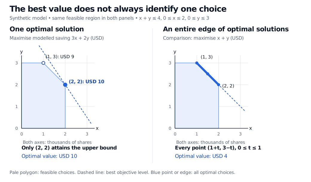
Two plots of the same synthetic feasible routing polygon. For savings 3x plus 2y, the unique optimal allocation is (2,2), worth USD 10; feasible allocation (1,3) is worth USD 9. Changing savings to x plus y gives USD 4 at every point of the edge from (1,3) to (2,2). Both axes measure thousands of shares.
The blue point or edge marks all optimal choices. Dashed lines show the best objective level. The right panel changes only the savings coefficients to USD 1 per thousand shares on each route.
When the best answer is a set
Keep all constraints but change the objective to x+y: both routes now save USD 1 per thousand shares. The best possible saving is USD 4, achieved whenever the total allocation is four thousand shares. The caps restrict the optimal choices to
(x,y)=(1+t,3−t),0≤t≤1.
This includes (1,3), (1.5,2.5) and (2,2), and every point between them. The optimal value is one number, USD 4; the set of optimal solutions is an entire edge. A solver returning one endpoint has not proved that the endpoint is uniquely best. A further preference, such as execution reliability, needs an explicit tie-break rule or a revised model.
What an optimality claim actually covers
“Optimal” is always relative to the stated objective, constraints and input assumptions. This model holds per-unit savings constant and omits market impact, fill uncertainty and lot-size restrictions. Its optimum does not promise realised savings or establish the best real execution plan.
A local optimum need only beat nearby feasible choices. In this linear example the feasible set is convex, and any local maximiser is global; uniqueness still needs the separate argument above. In a nonconvex problem, a solver can stop at a local solution that another feasible point beats. Numerical results also need a stated feasibility and optimality tolerance: a displayed rounded value alone is not an exact certificate.
Finally, a best finite bound need not be attained. Maximising q on 0≤q<1 has supremum 1, but no optimal solution: every allowed q can be improved to (q+1)/2. Our routing model avoids this issue because its feasible set is nonempty, closed and bounded and its objective is continuous, so a maximum is attained.
For the next mathematical step, Constrained and Convex Optimisation develops local versus global guarantees and optimality conditions (full lesson requires membership; public preview available).
Sources
Cornuéjols, G., Peña, J. and Tütüncü, R. Optimization Methods in Finance, 2nd edition, Cambridge University Press, 2018. Chapter 1, “Overview of Optimization Models,” defines feasible solutions, optimal solutions and optimal values; §§2.2 and 2.5 develop graphical linear optimisation and dual bounds.
Bertsimas, D. Geometry of Linear Optimization, MIT 15.093, Fall 2009, slides 7–8 and 21–23: unique and multiple solutions, feasible polyhedra and optimal corners.