A local optimum resists nearby feasible improvements. Distinguish minima from maxima, parameter choices from values, and genuine local optimality from a numerical stopping message.
Local optimum
A local optimum is a feasible choice whose objective function cannot be improved by sufficiently small feasible changes. For a minimisation problem it is a local minimum; for a maximisation problem it is a local maximum. The word local limits the comparison to a neighbourhood. A much better choice may exist elsewhere.
This matters when a quant researcher tunes model parameters: an optimisation routine can settle near a choice that resists nearby improvements without finding the best allowed parameters. Even a genuine global optimum would optimise the specified research objective, rather than establish future investment performance.
State the direction, the feasible choices, and the neighbourhood
Let D⊆Rn be the feasible set, and let f:D→R be the objective. For minimisation, a feasible point x∗ is locally optimal if there is a radius ε>0 such that
f(x∗)≤f(x)for every x∈D with ∥x−x∗∥2<ε.
For maximisation, reverse the inequality. Here the norm measures Euclidean distance between parameter choices; with one variable it reduces to absolute distance. Only feasible neighbours count. Infeasible parameter values cannot disprove constrained local optimality.
The choicex∗ and the objective valuef(x∗) are different objects. “Locally optimal at x=−1 with value 2” reports both. A reported value alone does not identify the parameters, and multiple choices can share a value.
The inequalities above allow ties. A strict local optimum requires a strict inequality for every other feasible point sufficiently close to x∗. The point itself must be excluded. For a constant objective on a real interval of positive length, every point is both a local minimum and a local maximum, and none is strict. Strictness distinguishes a nearby tie from a definite deterioration; it does not certify global superiority.
One curve, two directions, four useful comparisons
Consider an original toy research objective
f(x)=x3−3x,−3≤x≤3.
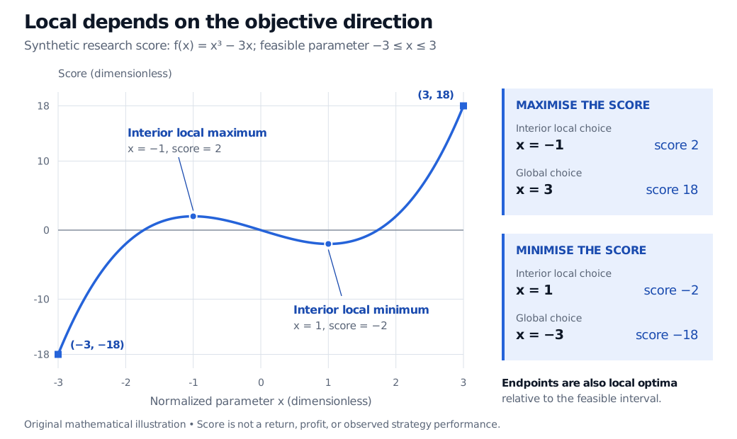
Both the normalised parameter x and the score are dimensionless. Suppose a researcher wants to maximise this score. It is a mathematical illustration of parameter search, not observed strategy returns, profit, or a calibrated performance measure.
At x=−1, the score is 2. Every sufficiently small nonzero change lowers it. That makes −1 a strict local maximiser. Nevertheless, x=3 scores 18. The nearby peak is not the best feasible choice.
The same curve also contains a strict interior local minimiser at x=1, with value −2. That point would matter if the task were to minimise f. It does not solve the researcher's maximisation problem.
Direction
Interior local choice
Its value
Global choice on [−3,3]
Its value
Maximise f
−1
2
3
18
Minimise f
1
−2
−3
−18
Synthetic dimensionless score x cubed minus 3x on the feasible interval from minus 3 to 3. The interior local maximum is at minus 1 with score 2, and the interior local minimum at 1 with score minus 2. Global maximum is at 3 with score 18; global minimum at minus 3 with score minus 18. The endpoints are also locally optimal relative to the interval.
Original synthetic objective. The cards separate each parameter choice from its score and compare the appropriate local and global answers for each direction.
To check the two interior claims directly, write the change as h:
For the global comparison, f′(x)=3(x−1)(x+1) is positive on (−3,−1), negative on (−1,1), and positive on (1,3). Comparing the endpoints and the two stationary values therefore gives the global answers in the table.
Under the feasible-neighbourhood definition used here, the endpoints are also strict local optima: −3 is a local minimum and 3 a local maximum. Their global status implies their local status. Some introductory calculus texts reserve “local extremum” for interior points; the convention here includes boundaries and suits constrained optimisation. The table identifies the interior local choices, rather than claiming they are the only local optima.
A common software mistake is to reverse the direction incorrectly. If a solver minimises, maximise the research score by giving it L(x)=−f(x). The local maximiser x=−1 of f becomes a local minimiser of L with value −2. Minimising f itself instead targets a different problem.
A stopping message is weaker than local optimality
For a differentiable objective, an interior local optimum must be a stationary point. That condition is necessary, not sufficient: g(x)=x3 has g′(0)=0, yet arbitrarily close negative and positive inputs give values below and above g(0). Zero is neither a local minimum nor a local maximum.
Conversely, boundary optima need not have a zero derivative. In the worked example, f′(−3)=f′(3)=24. The directions that would improve their respective objectives lie outside the feasible interval.
A numerical stopping rule may detect small steps, small objective changes, or an approximately zero gradient. Those are useful diagnostics, but each needs interpretation. They do not alone prove the mathematical neighbourhood inequality. Checking several starting points can reveal a better result; failure to find one does not prove that none exists.
Structure can provide a stronger conclusion. Minimising a convex function over a convex feasible set makes every local minimum global. For maximisation the corresponding condition is a concave objective over a convex feasible set. The cubic above lacks either guarantee over the whole interval. Even when such a guarantee holds, the chosen data, objective and constraints still determine what “best” means.
For derivative classification and search methods, Unconstrained Optimisation develops the multivariable tests. Constrained and Convex Optimisation explains boundary conditions and the local-to-global guarantee. Both have public previews; full lessons require membership.
Sources
Gérard Cornuéjols, Javier Peña and Reha Tütüncü, Optimization Methods in Finance, second edition (2018), §20.3, “Optimality Conditions”: local feasible-neighbourhood comparisons and necessary and sufficient conditions.