A stationary point has zero derivative or gradient. Learn why a flat tangent can mark a minimum, a maximum or neither—and what that means for optimisation.
Stationary point
A stationary point is a point where a function's derivative exists and equals zero. For a differentiable function of several variables, it is a point where the entire gradient is zero. In one variable the graph has a horizontal tangent there; it need not turn around.
That last distinction matters when minimising a pricing-error or strategy-research objective function. Solving “derivative equals zero” finds candidates for an optimum. It does not tell you which candidates are minima, or whether the best feasible answer is among them.
Flat at a point, still increasing
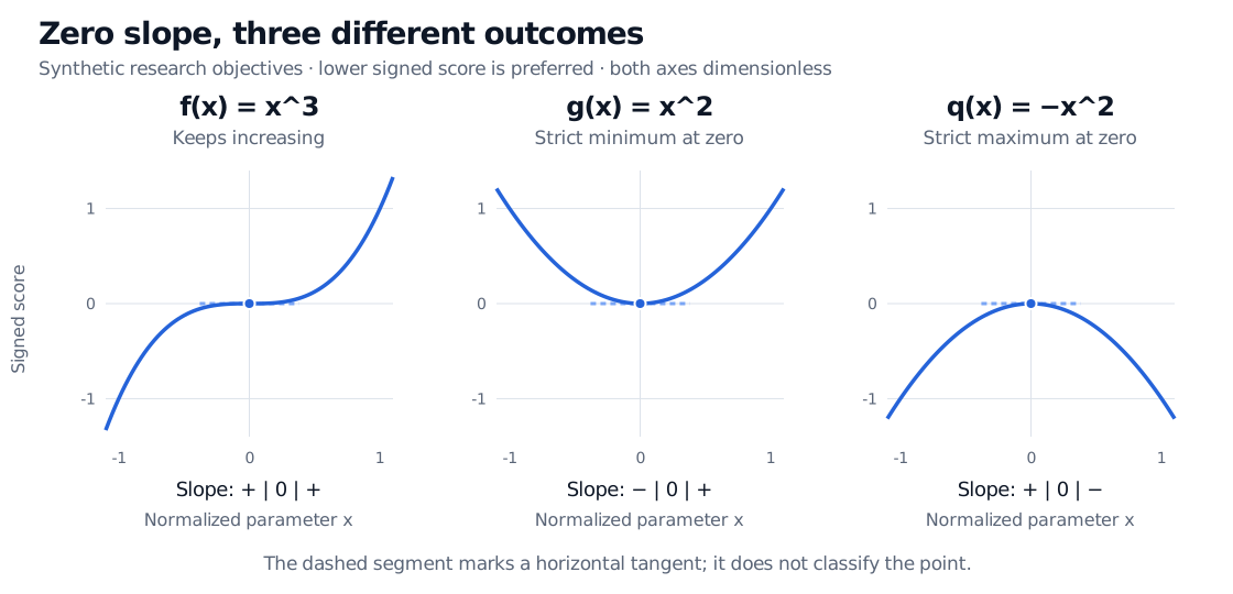
Suppose a researcher changes a model parameter around a reference value. Let x be the parameter displacement divided by a fixed positive scale, so x is dimensionless. Consider three hypothetical signed research scores, all dimensionless and all to be minimised:
f(x)=x3,g(x)=x2,q(x)=−x2.
These are synthetic shapes for learning about optimisation, not estimated market relationships. A signed score may be negative; it is not necessarily a squared-error loss.
At x=0, each score is zero and each first derivative is zero:
f′(x)=3x2,g′(x)=2x,q′(x)=−2x.
Yet their behavior differs:
For g, every nonzero displacement raises the score. Zero is a strict local minimum, and also the global minimum on the real line.
For q, every nonzero displacement lowers the score. Zero is a strict local maximum, the wrong answer for minimisation.
For f, negative displacements lower the score and positive ones raise it. In particular, f(−0.1)=−0.001 and f(0.1)=0.001. Zero is neither a minimum nor a maximum.
Three synthetic dimensionless research scores, x cubed, x squared and minus x squared, all have zero derivative at zero. The cubic keeps increasing; x squared has a strict minimum; minus x squared has a strict maximum. Dashed segments mark horizontal tangents.
Original synthetic objectives on identical scales. Zero slope is shared; turning behavior is not. Scores and normalized parameter x are dimensionless.
The cubic is strictly increasing, despite its zero derivative at zero. One direct proof is that, for a<b,
b3−a3=(b−a)(a2+ab+b2)>0.
The second factor equals (a+b/2)2+3b2/4 and can vanish only if a=b=0, which is excluded by a<b. Thus zero derivative at an isolated point does not contradict strict increase. Here f′′(x)=6x changes sign across zero, so the stationary point is also an inflection point.
What the condition actually says
For a differentiable function, stationarity at an interior point a means
f′(a)=0,f(a+h)−f(a)=o(∣h∣).
The notation on the right says that the change divided by ∣h∣ tends to zero as h→0. The first-order change disappears; higher-order changes remain. For the cubic at zero, the exact change is h3. There is no claim that the function is constant nearby.
An interior local minimum or maximum of a differentiable function must be stationary. The converse fails, as the cubic demonstrates. At a stationary point, a positive second derivative gives a strict local minimum and a negative one gives a strict local maximum, assuming the function is twice differentiable there in the usual neighborhood sense. If the second derivative is zero, that test is inconclusive: x4 has a strict minimum at zero, while x3 has neither extremum.
Terminology needs care. Many calculus texts use critical point more broadly to include a point in the function's domain where the derivative does not exist. Under that convention, ∣x∣ has a critical minimum at zero but no stationary point there. Some optimisation texts use “critical” as a synonym for stationary after assuming differentiability. Check the stated convention.
Boundary solutions also need separate attention. Minimising f(x)=x over [0,1] gives the unique global minimum at zero, although the derivative of the underlying function is 1. The useful direction of movement lies outside the permitted interval.
Before accepting a solver's answer
A solver that stops because its gradient is small has met a numerical stationarity tolerance; that alone certifies neither a local nor a global minimum. Scaling the parameter or score changes the numerical gradient and therefore the meaning of an absolute tolerance.
Check feasible nearby changes and the relevant curvature. With several parameters, ∇f(x)=0 means that every first-order directional change vanishes, assuming differentiability. Curvature can still reveal a descending direction: a saddle point is stationary without being a local optimum. The Hessian matrix organises those second-order effects.
Unconstrained Optimisation develops these gradient and Hessian tests alongside descent methods. Its outline is public; the full lesson requires membership.
Sources
Gérard Cornuéjols, Javier Peña and Reha Tütüncü, Optimization Methods in Finance, second edition (2018), §20.3, Theorems 20.1–20.2: first-order necessary and second-order sufficient conditions for unconstrained minimisation.