A derivative is a local rate of change and tangent slope. Translate a bond price derivative into a basis-point estimate, keeping units and finite-move error explicit.
Derivative (calculus)
A derivative is a function's instantaneous rate of change with respect to an input. For a price expressed as a function of yield, it measures the local price sensitivity to yield. Geometrically, it is the slope of the tangent line at the chosen point.
The word also names a financial derivative, such as an option or a swap. That is a contract. A calculus derivative is a mathematical rate of change; it can describe a contract's sensitivity, but the two meanings are distinct.
From an observed change to a limiting slope
Suppose an input changes from a to a+h, with h=0. The difference quotient
hf(a+h)−f(a)
is the average change in the output per unit change in the input over that step. It is the slope of the secant through the two points on the graph.
At an interior point of the domain, the ordinary derivative is the limit
f′(a)=h→0limhf(a+h)−f(a),
provided this two-sided limit exists as a finite real number. The step approaches zero through nonzero values; substituting h=0 directly would give an undefined quotient. Positive and negative steps must approach the same slope. At a domain endpoint, one may instead specify a one-sided derivative.
The notation f′(a) denotes a number at one point. Allowing the point to vary gives a new function f′(x), defined wherever the derivative exists. Other common notation is df/dx. The output unit is always the original output unit divided by the input unit. OpenStax §3.1 develops this connection between secants, tangent slopes and rates of change.
A yield move is small only after its units are specified
Consider a hypothetical zero-coupon bond paying USD 100 exactly two years from today. Hold the payment and maturity fixed, ignore credit and trading costs, and use a single annual continuously compounded yield y, entered as a decimal. Its present value is
P(y)=100e−2yUSD.
Here y=0.05 means 5% per year. Differentiating the exponential, including the inner factor −2 from the chain rule, gives
P′(y)=−200e−2y=−2P(y).
At the starting yield,
P(0.05)=90.48374180USD,P′(0.05)=−180.96748361USD per unit of decimal yield.
The minus sign says that increasing yield decreases this fixed payment's discounted price. The magnitude is a rate, not the price loss from every yield move. One basis point is 0.0001 in decimal yield, so a one-basis-point rise gives the first-order estimate
These agree closely, but they are different calculations. Exact repricing uses both endpoint prices. The derivative estimate uses only the initial slope.
The units also explain a common factor-of-100 error. If the yield input is instead the percentage number u=100y, so the starting input is u=5, then dP/du=P′(y)/100=−1.80967484 USD per percentage point at that point. It describes the same curve in different input coordinates. Multiplying the decimal-yield derivative by a step of 1 when the intended step was one basis point exaggerates the estimated change by a factor of 10,000.
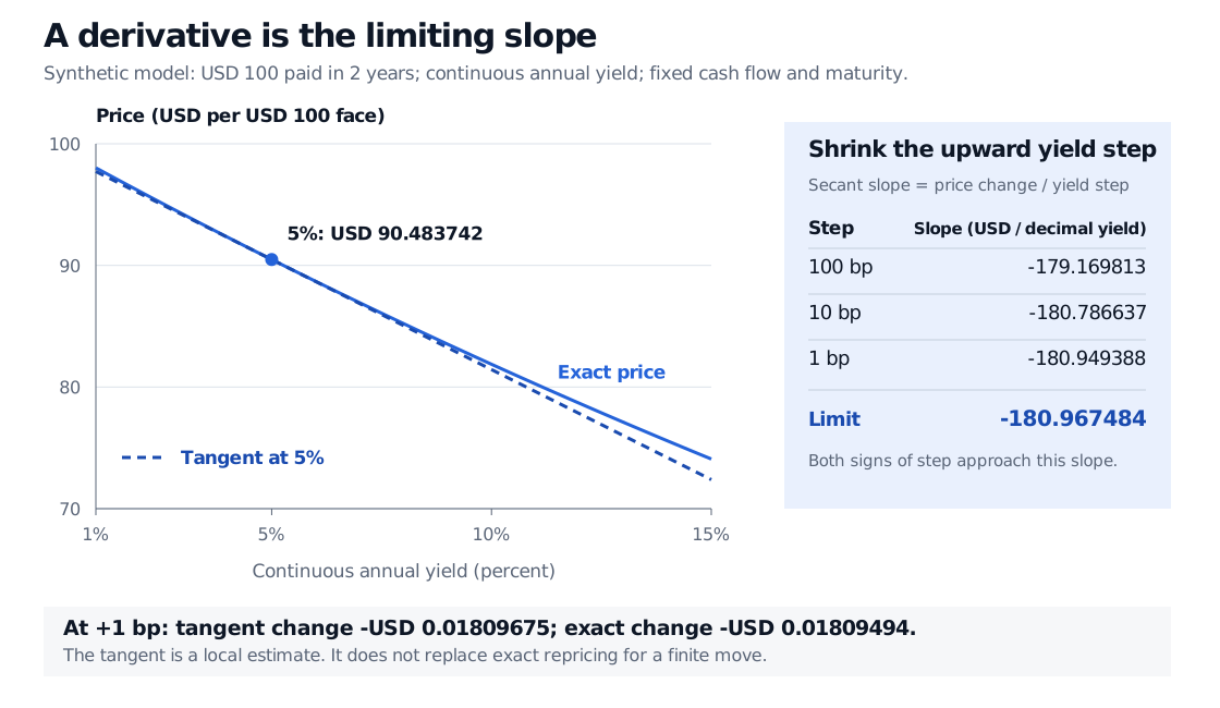
Synthetic two-year USD 100 payment: at 5% continuous yield the price is USD 90.483742 and its tangent slope is minus 180.967484 USD per decimal yield. Upward-step secant slopes for 100, 10 and 1 basis point are minus 179.169813, minus 180.786637 and minus 180.949388, converging toward the derivative.
Original synthetic example. Fixed USD 100 payment in two years, continuous annual yield. The price curve and its tangent agree locally; shrinking secant steps recover the tangent's slope.
What the tangent promises
The tangent line at a is
L(a+h)=f(a)+f′(a)h.
Differentiability says more precisely that
f(a+h)=f(a)+f′(a)h+r(h),h→0limhr(h)=0.
The approximation error becomes small relative to the input step. This statement provides no universal threshold for a sufficiently small move and no numerical error bound for a specified finite move. OpenStax §4.2 explains the tangent approximation and its use for small changes.
For the bond, increasing yield by 100 basis points, from 5% to 6%, produces a tangent estimate of −USD 1.80967484, compared with an exact change of −USD 1.79169813. The second derivative is P′′(y)=4P(y)>0 throughout this model, so the price curve is convex and lies above its tangent: the initial slope overstates the loss on a yield rise. A first derivative alone does not encode that curvature.
A derivative need not exist everywhere. For f(x)=∣x∣, the left slope at zero is −1 and the right slope is +1; there is no single derivative there, despite continuity. A kinked payoff therefore needs care at its kink. In a model with several varying inputs, a partial derivative specifies which input changes while the others are held fixed; one sensitivity does not explain every source of a realised price change.
For a relative rather than a dollar sensitivity, logarithmic differentiation works with P′/P, which is −2 in this continuous-yield example. In the reverse direction, an antiderivative recovers a function from its derivative, with a constant fixed by a known value.
James Stewart, Single Variable Calculus: Early Transcendentals, 6th edition, §§2.7–2.8 and 3.10: derivative limits, derivative functions and tangent approximations.
John C. Hull, Options, Futures, and Other Derivatives, 9th Global Edition, §4.2, “Continuous Compounding”: exponential accumulation and discounting conventions.