Understand partial derivatives as fixed-input sensitivities, calculate portfolio variance changes, and distinguish an allocation partial from a total derivative.
Partial derivative
A partial derivative measures how a function changes with one input while its other independent inputs are held fixed. For a portfolio risk model, it can answer “how sensitive is variance to correlation at these weights?” For an option price, delta asks the corresponding question about the underlying price.
The phrase held fixed is part of the definition. A partial derivative describes a controlled change in a model; it does not predict that other market inputs will stay unchanged.
Turn a surface into a curve
For a multivariable functionf(x,y), the partial derivative with respect to x at (a,b) is
∂x∂f(a,b)=h→0limhf(a+h,b)−f(a,b),
provided the limit exists. The second coordinate stays at b throughout. Fixing it gives an ordinary function of one variable, x↦f(x,b), and the partial derivative is that curve's derivative.
The notation fx means the same thing as ∂f/∂x. To compute it, apply the usual differentiation rules while treating y as constant. For example, if f(x,y)=x2y+3y, then fx=2xy whereas fy=x2+3. A term constant in one calculation can vary in the other.
Two levers on the same portfolio
Consider a synthetic portfolio held over one period. Its two assets have simple returns measured as decimals, with standard deviations 0.20 and 0.10 over that same period. Let w be the initial weight in asset A and 1−w the initial weight in asset B. Assume no interim rebalancing, and write their return correlation as ρ.
The covariance is ρ(0.20)(0.10). For this long-only illustration, 0≤w≤1 and −1≤ρ≤1. The inputs are stipulated scenarios, rather than estimates or investment recommendations.
Here vw changes the allocation while holding correlation fixed: increasing w automatically reduces B's weight. It does not hold B's weight fixed. We already built the fully invested budget into the coordinates by substituting wB=1−w. Differentiating a model with separate independent coordinates wA,wB would answer a different question.
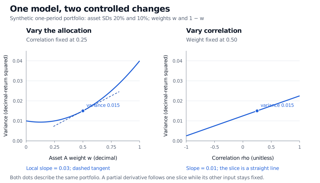
Two slices of the synthetic portfolio variance model. With correlation fixed at 0.25, varying weight gives a curved slice with slope 0.03 at weight 0.50. With weight fixed at 0.50, varying correlation gives a straight line of slope 0.01. Both selected points have variance 0.015.
Original synthetic one-period model. The output is variance of decimal returns. The two dots represent the same input pair; each curve changes only one coordinate.
A sensitivity is not a finite change
A derivative must be multiplied by an input change. Raising A's weight from 50% to 51% is Δw=0.01, not 1. Raising correlation from 0.25 to 0.35 is Δρ=0.10. At the baseline above:
Controlled change
First-order variance change
Exact variance change
New variance
w:0.50→0.51, correlation fixed
0.03(0.01)=0.000300
0.000304
0.015304
ρ:0.25→0.35, weights fixed
0.01(0.10)=0.001000
0.001000
0.016000
The allocation slice curves, so its tangent estimate has a small error. The correlation slice is linear at fixed weights, so that estimate is exact throughout the allowed correlation interval. At w=0 or w=1, vρ=0: correlation cannot change the variance of a portfolio holding just one asset.
The derivative's units are output units per input unit. Here they are decimal-return squared per unit of weight or correlation. Neither 0.03 nor 0.01 is itself a percentage change in portfolio risk.
If both inputs move, specify the path
Suppose a stress scenario explicitly makes correlation depend on the allocation: ρ=ρ(w). The chain rule gives a total derivative along that path:
dwdv(w,ρ(w))=vw(w,ρ(w))+vρ(w,ρ(w))ρ′(w).
For the chosen local path ρ(w)=0.25+2(w−0.50), the slope at w=0.50 is
0.03+0.01(2)=0.05.
Use this path only where both inputs remain within their stated domains. It is an imposed scenario relationship, not a claim that trading a weight causes market correlation to change. The partial derivative remains 0.03 at the baseline; 0.05 answers the different question in which correlation moves too.
More generally, for small independently specified bumps, differentiability gives
Δv≈vwΔw+vρΔρ.
The gradient collects those partials. If both table changes occur together, the estimate is 0.001300, while direct evaluation gives 0.0013036. Curvature and interaction terms explain the residual. A full scenario recalculation retains them.
Variance sensitivity and volatility sensitivity differ
At our baseline, s=0.015≈0.122474, or 12.2474% over the specified period. Its weight sensitivity is approximately 0.122474 decimal-return units per unit weight. A one-percentage-point increase in A's weight therefore raises standard deviation by approximately 0.1225 percentage points locally. This is different from the variance change of 0.000300.
At zero variance, the division above is unavailable; differentiability of the square root composite needs separate analysis. At domain boundaries, two-sided bumps may also be infeasible: use admissible one-sided comparisons rather than evaluating invalid correlations or forbidden weights. The polynomial's formula can exist outside a portfolio model's economically allowed domain without making those scenarios permissible.
The Partial Derivatives lesson develops fixed-input sensitivities, gradients and higher partials with worked examples. Its public page is a preview; the full lesson requires membership.
Sources
Stanford University Mathematics Department, Linear Algebra, Multivariable Calculus, and Modern Applications, Math 51 course text, version last modified 10 March 2021, Chapter 9, especially Definition 9.2.2 and §9.3. Defines coordinate slices and the partial derivative; the portfolio scenario and figure here are original.