A multivariable function maps several inputs to one scalar output. Read a bond-value contour, hold inputs fixed, and separate remaining maturity from passing time.
Multivariable function
A multivariable function takes an ordered collection of inputs and assigns one output to each allowed input collection. Here the output is a real number, so the function is scalar-valued:
f:D⊆Rn→R,(x1,…,xn)↦f(x1,…,xn),n≥2.
The domain specifies the allowed input combinations. “Multivariable” describes the number of inputs; it does not mean several outputs. Functions with vector outputs are a further generalisation.
In finance, a single valuation can depend on yield, maturity and cash flows at once. A one-input chart shows only a slice of that relationship. Keeping track of which inputs are free to change is the first step toward interpreting a price sensitivity correctly.
Two inputs behind one bond value
Consider a hypothetical certain payment of USD 100, with no intermediate coupons. Its present value under continuous discounting is
V(y,T)=100e−yT,
where y is a continuously compounded annual yield expressed as a decimal, and T is remaining maturity in years. Thus 5% means y=0.05, not 5. The product yT is dimensionless and V is in USD. The payment amount is fixed as a parameter in this two-input function; allowing it to vary would give a three-input function.
At y=0.05 and T=2,
V(0.05,2)=100e−0.1≈90.4837.
The exponential expression is mathematically defined for every real pair (y,T). For this payment interpretation we restrict the domain to y∈R and T≥0. Negative yields are allowed: for T>0, a negative yield makes this model value exceed USD 100. At maturity, T=0 gives exactly USD 100 for every yield.
This is a discounting model for a specified certain cash flow. Using it as a market price requires an appropriate discount rate and consistent financing assumptions. A real coupon bond has several dated payments; credit risk, liquidity and the term structure can require richer inputs. When comparing maturities here, we deliberately allow y and T to vary separately rather than imposing an observed yield curve y(T).
Reading the contours
The graph of V(y,T) is a surface: two coordinates locate the inputs and a third gives the USD output. A contour plot places equal-value curves in the two-dimensional input plane. Formally, the level set at value c is
Lc={(y,T)∈D:V(y,T)=c}.
For 0<c<100 and positive yields and maturities, the condition becomes
yT=−ln(c/100).
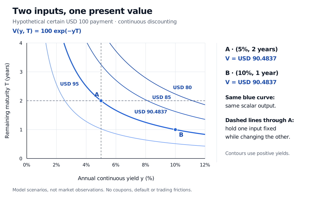
Yield–maturity contours for a certain USD 100 payment discounted continuously. Point A at 5% yield and 2 years and point B at 10% yield and 1 year both have value USD 90.4837. Other curves show USD 80, 85 and 95. Dashed lines through A hold one input fixed.
Original hypothetical continuous-discounting model. Yield is an annual percentage on the axis; maturity is remaining years. Curves join equal USD values; dashed lines hold one input fixed. No coupons, default or trading frictions.
Points A and B share yT=0.1, so they produce the same value. This does not violate the definition of a function: each input pair has one output, but different input pairs can share an output. Knowing the value alone does not identify both inputs.
The dashed lines answer different questions from the contours. A horizontal dashed line fixes T=2 and changes yield. A vertical dashed line fixes y=5% and changes remaining maturity. Moving along a contour generally changes both inputs together.
A sensitivity needs a “held fixed” instruction
A partial derivative changes one input while holding the others fixed. For this function,
∂y∂V=−TV,∂T∂V=−yV.
At point A these are approximately −180.9675 USD per unit of the decimal annual-yield input and −4.5242 USD per additional year of remaining maturity. The first number is not the dollar effect of a one-percentage-point yield move. For a one-basis-point increase, Δy=0.0001, the local estimate is
ΔV≈(−180.9675)(0.0001)=−0.01810 USD.
Exact revaluation gives approximately −0.01809 USD. A derivative is an instantaneous slope, so a finite bump need not match its first-order estimate exactly.
Remaining maturity and calendar time run in opposite directions. At positive yield, adding remaining maturity lowers this value. But one day passing reduces T by 1/365 under an ACT/365 convention. Holding yield fixed, that raises the value by about USD 0.01240 in this example. The negative ∂V/∂T therefore does not imply that the value falls as the clock advances. At negative yield, the maturity sensitivity reverses sign.
If yield and maturity both change, the first-order estimate combines the two partial effects:
ΔV≈−TVΔy−yVΔT.
The gradient collects those partial derivatives. For large changes, revalue the function directly rather than assuming the local estimate remains accurate. For a path on which yield itself depends on time, the chain rule accounts for that dependence.
Several inputs need not be certain—or independent
The rule V(y,T) is deterministic: once its inputs are specified, its output is fixed. Its inputs can nevertheless be uncertain. Feeding a random future yield into the same function makes the resulting future value random. The function alone does not specify that yield's distribution or make its inputs statistically independent.
This distinction separates two modelling tasks: choosing how a given scenario maps to a value, and choosing which scenarios can occur. Both matter in risk analysis.
For a fuller treatment of fixed-input slices, gradients and simultaneous changes, see Partial Derivatives — Mathematics Primer. The public page is a preview; the full lesson requires membership.
Sources
Steven G. Krantz and Harold Parks, Vector Calculus, 1st edition, CRC Press, 2024, §3.1, especially Definition 3.1.1 and §3.1.2 on graphs and level sets.
John C. Hull, Options, Futures, and Other Derivatives, 9th edition, Global Edition, §§4.2–4.4 on continuous compounding, zero rates and bond pricing. The numerical example and figure above are original.