Differentiate a composition by multiplying its local sensitivities. Trace a factor through a discount rate to a bond price, with the inner derivative and units intact.
Chain rule
The chain rule differentiates a composite function: one function applied to the output of another. It multiplies the outer function's local sensitivity by the inner function's local sensitivity. In finance, that converts exposure to a pricing input into exposure to the factor that moves that input.
If y=f(u) and u=g(x), then
dxdy=f′(g(x))g′(x)=dudydxdu.
This holds when g is differentiable at x and f is differentiable at g(x). Evaluate the outer derivativeat the inner value, then multiply by the inner derivative. The notation resembles cancelling du, but the result is a theorem about differentiable functions, not permission to cancel arbitrary derivative symbols. OpenStax, §3.6, gives the rule and its conditions.
A factor moves a rate, and the rate moves a price
Consider a hypothetical zero-coupon bond paying a certain USD 100 in exactly two years. Its present value, using a continuously compounded annual discount rate r expressed in decimals, is
P(r)=100e−2r.
Suppose a dimensionless model factor x determines that rate through
r(x)=0.03+0.5x.
The cash flow and two-year maturity stay fixed. This is an assumed scenario mapping, not an estimated market relationship. At x=0.04, the rate is r=0.05, or 5% per year, and
P=100e−0.1≈USD 90.483742.
There are two links to differentiate:
drdP=−2P,dxdr=0.5.
Therefore,
dxdP(r(x))=drdPdxdr=(−2P)(0.5)=−P≈−90.483742.
The answer is USD per unit of x. The intermediate sensitivity dP/dr≈−180.967484 is USD per unit of annual decimal rate. Multiplying by the rate loading 0.5 converts it to exposure to x.
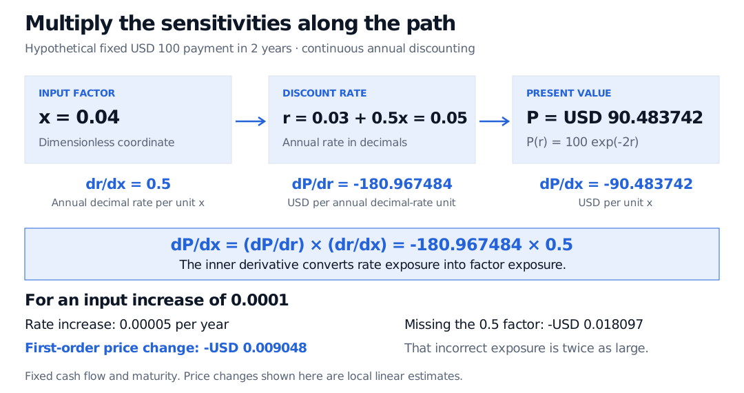
A dimensionless factor x of 0.04 maps to an annual decimal rate of 0.05 and present value USD 90.483742. The price-rate sensitivity is minus 180.967484; multiplying by the rate loading 0.5 gives minus 90.483742 USD per unit x. Omitting 0.5 doubles the exposure.
Original hypothetical sensitivity diagram. The certain USD 100 payment and two-year maturity are fixed; discounting is continuous. Bottom-panel price changes are first-order estimates.
For an input increase Δx=0.0001, the rate increases by 0.00005, or half a basis point. The first-order estimate is
ΔP≈dxdPΔx=−90.4837418(0.0001)≈−USD 0.009048374.
Repricing exactly at x=0.0401 gives USD 90.474694, a change of approximately −USD 0.009047922. The small difference arises because the derivative gives a local linear approximation to a curved price function.
Forgetting dr/dx=0.5 would produce an estimated change of −USD 0.018096748, twice the correct first-order exposure. It would answer the rate-bump question while using the factor's bump size.
Find the layers before differentiating
For the bond example, substitution gives an independent way to see the same answer:
P(r(x))=100e−2(0.03+0.5x)=100e−0.06−x.
Differentiating the last expression yields −100e−0.06−x=−P. The two approaches agree because they describe the same function.
where the expressions and required derivatives exist. With three layers, f(g(h(x))), multiply three local derivatives: f′(g(h(x)))g′(h(x))h′(x). Identifying the layers first makes omitted factors easier to catch. See MIT's chain-rule explanation for further composition examples.
Units also reveal hidden layers. If a screen displays the rate as q=100r, so that q=5 means 5%, then dr/dq=0.01 and dP/dq=0.01dP/dr. A sensitivity per percentage point differs from one per unit of decimal rate. Always specify the coordinate being bumped.
When there is more than one route
For differentiable functions V, a and b, if V(a,b) depends on two inputs that both respond to x, the total derivative adds the contributions from both routes:
dxdV(a(x),b(x))=∂a∂Va′(x)+∂b∂Vb′(x).
Each partial derivative holds the other pricing input fixed. If only a responds to x, then b′(x)=0 and the second route contributes nothing. A risk report must state which inputs move together; the chain rule propagates that specified mapping without establishing that it is causal.
Finally, differentiating a pricing formula with respect to a scenario input is different from transforming an entire stochastic price process. Brownian paths are not ordinary differentiable time paths. Itô's lemma includes a second-derivative correction driven by quadratic variation; the ordinary first-derivative chain alone is insufficient for that task. Tehranchi's notes, Chapter 2, §§3–4, explain the distinction.
James Stewart, Single Variable Calculus: Early Transcendentals, 6th edition, §3.4, “The Chain Rule”: differentiability conditions, evaluated outer derivative and repeated composition.
John C. Hull, Options, Futures, and Other Derivatives, 9th Global Edition, §4.2, “Measuring Interest Rates”: continuously compounded rates and discounting.