Differentiate products, quotients and variable powers through logarithms; connect the relative derivative to bond yield sensitivity, with domain and finite-change limits.
Logarithmic differentiation
Logarithmic differentiation finds a derivative by taking the natural logarithm of a function, simplifying with log laws, then differentiating and multiplying back by the original function. It is especially useful for products, quotients and variable powers. In finance, the intermediate result often has its own meaning: a sensitivity relative to the current value.
First find the relative slope, then recover the slope
For a differentiable real function f that is nonzero near the point of interest, the chain rule gives
dxdln∣f(x)∣=f(x)f′(x),f′(x)=f(x)dxdln∣f(x)∣.
The ratio f′/f is the logarithmic derivative. The method is to make the log expression easier first, differentiate it, and multiply by f, including its sign. Forgetting that last multiplication returns a relative sensitivity instead of the requested level derivative. OpenStax §3.9 develops the method through log laws and implicit differentiation.
For example, on an interval where u and v are positive, let f=ua/vb, with constant real exponents a,b. Then
lnf=alnu−blnv⟹f′=vbua(auu′−bvv′).
Each factor contributes its own relative slope; the quotient contributes a minus sign. This is the same calculus as the product and quotient rules, rearranged to exploit the expression's structure.
When both base and exponent vary, write f(x)=g(x)h(x) with g(x)>0. Taking logs gives lnf=hlng, so the product rule yields
f′=gh(h′lng+hgg′).
Using only the constant-exponent power rule would omit h′lng. For a general real-valued variable power, positivity of the base is what makes gh=exp(hlng) a well-defined real differentiable expression.
A USD 100 payment becomes a yield sensitivity
Consider a hypothetical zero-coupon bond paying USD 100 exactly three years from today. Hold the payment and its date fixed. Under an annual effective yieldy>−1, its present value is
V(y)=(1+y)3100USD.
Taking the log of value divided by its USD 100 face amount keeps the logarithm's argument dimensionless:
ln(100USDV(y))=−3ln(1+y)⟹V(y)V′(y)=−1+y3.
At y=0.05, the price is USD 86.38375985 and the relative derivative is −3/1.05=−2.857142857. Multiplying back gives
V′(0.05)=−246.81074244USD per unit of decimal yield.
The negative of the relative derivative is the bond's modified duration, 2.857142857 years under this annual convention. It is not a dollar loss. Hull's §4.8 relates modified duration to small price changes for a specified compounding frequency; changing the yield convention changes the derivative.
One basis point is 0.0001 in decimal yield. For a rise from 5% to 5.01%, the first-order estimate is
That is approximately a 0.02857143% fall in price, not a 2.857% fall. CME's duration discussion distinguishes a one-basis-point dollar sensitivity from the relative sensitivity used in duration.
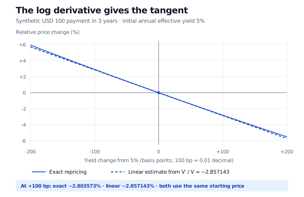
Exact repricing gives a loss of USD 0.02467637. For a larger rise from 5% to 6%, the linear estimate is −USD 2.46810742, while exact repricing gives −USD 2.42183155. The derivative is exact at the original yield; using it for a finite move introduces approximation error.
Exact relative price change and its tangent estimate for a hypothetical three-year USD 100 zero-coupon bond initially yielding 5% annually effective. At a 100-basis-point rise, the exact price fall is 2.803573%, versus the linear estimate of 2.857143%. At a 200-basis-point rise the falls are 5.503317% and 5.714286%.
Synthetic fixed-payment example: USD 100 in three years, initial annual effective yield 5%. The tangent uses the logarithmic derivative at the starting yield. The two curves agree locally and separate as the yield move grows.
This calculation isolates a yield change at one valuation instant. It includes no passage of time, coupons, default, trading costs or changing cash flows. A large move needs repricing or higher-order terms; changing promised cash flows requires a richer valuation model.
Where the logarithm is allowed
Writing lnf requires f>0. A negative function can still be handled with ln∣f∣ wherever it is nonzero. For example, f(x)=−x2 on x>0 gives ln∣f∣=2lnx, hence f′/f=2/x and f′=(−x2)(2/x)=−2x. Multiplying by ∣f∣ instead would get the sign wrong. University of Alberta's calculus notes state this absolute-value form explicitly.
If f is differentiable at an interior point and nonzero there, continuity keeps its sign unchanged in a sufficiently small neighbourhood. That is the local justification for the log step. At a zero, however, ln∣f∣ and f′/f are undefined even if f′ exists. For the same −x2, the derivative at zero is still zero, obtained separately. Likewise, splitting an expression into logs can exclude zeros of its individual factors. Check those points against the original function.
Absolute values do not enlarge the domain of the original expression: they cannot repair division by zero, an invalid real square root or an undefined real variable power.
Differentiation is not differencing
The local relation is
f(x)Δf≈f(x)f′(x)Δx.
The left side is a finite relative change; the derivative on the right describes its first-order behaviour as the move shrinks. For two positive observations, ln(V1/V0) is a finite log change. Dividing it by a finite input interval gives an average log slope, which need not equal the derivative at either endpoint. Taking logs of a market time series does not make the observed path differentiable.
James Stewart, Single Variable Calculus: Early Transcendentals, 6th edition, §3.6, pp. 217–219 — absolute-value logarithms, logarithmic differentiation and variable exponents.
John C. Hull, Options, Futures, and Other Derivatives, 9th Global Edition, §4.8, especially the “Modified Duration” subsection and equation 4.17 — yield conventions and local bond-price sensitivity.