Limit of a function: Definition & Examples

A limit of a function is the value its output approaches as its input approaches a specified point. The input gets close to the point without having to equal it. We write

\lim_{x\to a}f(x)=L.

This describes nearby behaviour, so it can be meaningful even when $f(a)$ is undefined. In finance, a limit can reveal the sensible zero-rate value of a cash-flow formula that appears to divide by zero.

“Approaches” is a requirement on every nearby input

For a real-valued function, the finite limit

L

means that any positive output tolerance can be met by restricting the input to a sufficiently small neighbourhood of

a

. More precisely, for every

\varepsilon>0

, there is a

\delta>0

such that

0<\lvert x-a\rvert<\delta \quad\Longrightarrow\quad \lvert f(x)-L\rvert<\varepsilon, \qquad x\in D,

where

D

is the function's domain. The point

a

must be an accumulation point of

D

: there must be admissible inputs arbitrarily close to it. The condition

0<\lvert x-a\rvert

deliberately excludes the value at

a

The word every matters. A few favourable inputs do not establish a limit. Nor must the output move monotonically towards

L

; it may fluctuate while staying inside successively smaller tolerances.

For the usual two-sided limit at an interior point, inputs approach from both directions. The condition is

\lim_{x\to a^-}f(x)=L \quad\text{and}\quad \lim_{x\to a^+}f(x)=L.

The minus superscript means $x<a$ ; the plus means $x>a$ . Both sides must exist and agree. At a domain endpoint, state the relevant one-sided limit explicitly rather than inventing inputs outside the domain.

A quotient with a hole

Consider the dimensionless function

g(y)=\frac{e^{2y}-1}{y},\qquad y\ne0.

Substitution at zero produces

0/0

, which is an indeterminate form, not an answer. Nearby evaluations give:

Negative input $y$	$g(y)$	Positive input $y$	$g(y)$
−0.01	1.9801327	0.01	2.0201340
−0.001	1.9980013	0.001	2.0020013
−0.0001	1.9998000	0.0001	2.0002000

The table suggests 2. An analytic argument explains why: for $y\ne0$ ,

g(y)=\int_0^2 e^{yt}\,dt.

For $0\le t\le2$ , the integrand lies between $e^{-2\lvert y\rvert}$ and $e^{2\lvert y\rvert}$ . Hence

2e^{-2\lvert y\rvert}\le g(y)\le2e^{2\lvert y\rvert}.

Both bounds tend to 2 as

y\to0

, which proves the limit by squeezing. This argument uses integration and the exponential function; the table alone is only evidence.

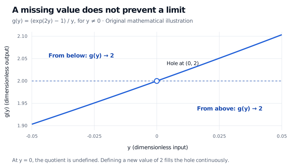
The dimensionless function g(y)=(exp(2y)−1)/y approaches 2 from below for negative y and from above for positive y. An open circle at (0,2) marks the undefined value at zero.

Original mathematical illustration. The quotient has a two-sided limit of 2 despite being undefined at zero.

Defining a new function with the same quotient away from zero and value 2 at zero makes a continuous extension. Assigning value 7 instead would leave the limit at 2 but fail continuity at zero. The limit and the point value answer different questions.

A cash-flow formula at zero interest

Suppose a hypothetical contract pays continuously at USD 6,000 per year for exactly two years. Use a constant, continuously compounded discount rate $r$ , measured per year and entered as a decimal; time $t$ is measured in years. Ignore credit risk, fees and taxes. This is an idealised continuous stream, not a monthly-payment annuity.

Its present value is the payment rate multiplied by a continuous annuity factor:

V(r)=6000A(r),\qquad A(r)=\int_0^2 e^{-rt}\,dt =\frac{1-e^{-2r}}{r},\quad r\ne0.

The factor has units of years, so USD per year multiplied by years gives USD. At exactly $r=0$ , use the integral: its integrand is 1 throughout the two years. Therefore

A(0)=2\ \text{years},\qquad V(0)=12000\ \text{USD}.

The nonzero-rate formula agrees with this limit. Numerically, its year-valued factor is

g(-r)

when

r

is entered in the stated annual units. At

r=0.001

per year, or 0.1% per year, the factor is approximately 1.9980013 years and present value is USD 11,988.01. At a negative rate of the same magnitude the factor exceeds two years. These comparisons follow from the assumed discount factors; a limit does not justify using a flat discount rate for every real contract.

For a general nonnegative horizon $T$ , the same reasoning gives $A(r)=(1-e^{-rT})/r\to T$ . A formula's apparent singularity may therefore be removable even though direct division at the exceptional input remains invalid.

Computing close to the point

The limit is a statement about real numbers. A computer stores approximations. For very small

y

, calculating exp(2*y) - 1 subtracts nearly equal numbers and can lose significant digits. Python's expm1(z) evaluates

e^z-1

directly with better precision near zero. This is a numerical stability issue, separate from whether the mathematical limit exists.

from math import expm1

def annuity_factor(r, years):
    return years if r == 0 else -expm1(-r * years) / r

print(expm1(2 * 0.001) / 0.001)
# 2.002001334000267
print(round(6000 * annuity_factor(0.001, 2), 2))
# 11988.01
print(6000 * annuity_factor(0, 2))
# 12000

The explicit zero branch implements the continuous extension. It does not perform a division by zero or prove the limit by numerical sampling.

Finally, not every missing point can be filled this way. For $f(x)=\lvert x\rvert/x$ , the left-hand limit at zero is −1 and the right-hand limit is 1, so no two-sided limit exists. For $1/x^2$ , the notation $\lim_{x\to0}1/x^2=+\infty$ describes unbounded growth, not a finite limiting value. Identify the behaviour before deciding whether a formula merely needs a value filled in.

Sources

Stewart, J. (2008). Single Variable Calculus: Early Transcendentals, 6th ed., §§2.2 and 2.4: nearby behaviour, one-sided limits and the precise definition.
Hull, J. C. (2018). Options, Futures, and Other Derivatives, 9th Global ed., §4.2: continuously compounded rates and exponential discounting.
OpenStax, Calculus Volume 1, §2.2: The Limit of a Function: one-sided versus two-sided limits and infinite limits.
Python documentation, math.expm1: accurate evaluation of the exponential minus one near zero.

“Approaches” is a requirement on every nearby input

A quotient with a hole

A cash-flow formula at zero interest

Computing close to the point

Sources

Related terms

Continuity

Definite integral

Domain of a function

Exponential function

Numerical stability

Present value