See why an exact formula can lose a quarter of a root in floating-point arithmetic, how to reformulate it, and why stability differs from conditioning.
Numerical stability
Numerical stability describes how well a computational procedure controls the effects of rounding and other small computational errors. A stable method avoids unnecessarily amplifying those errors beyond the sensitivity inherent in the mathematical problem. Two formulas can be identical in exact arithmetic and produce very different answers on a computer.
In finance, this matters when a calculation extracts a small return, hedge residual or price difference from larger intermediate values. A correct pricing identity does not by itself guarantee an accurate implementation. The relevant questions are how the answer was computed and how sensitive that answer is to its inputs.
Two formulas, one root
Consider the dimensionless synthetic quadratic
x2−108x+1=0.
Its roots are approximately 108 and 10−8. The usual formula evaluates the small root as
xsmall=2108−1016−4.
The square root is extremely close to 108. Rounding it before the subtraction leaves very little reliable information in the difference. This is catastrophic cancellation: errors already present in the nearly equal operands become large relative to their small difference. The subtraction itself can even be exact for the stored operands; the damage comes from the approximations it exposes.
The roots multiply to 1, so compute the large root using addition and recover the small one through its reciprocal:
The reference begins 1.0000000000000001000×10⁻⁸. The reformulation preserves essentially all the accuracy available in this arithmetic. It changes the route through the calculation while keeping the polynomial unchanged.
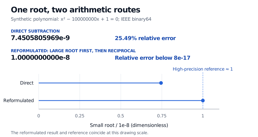
For a synthetic quadratic, the direct small root is 7.4505805969e-9, about 25.49% below the reference. The reformulated value 1e-8 overlaps the reference at the diagram's scale.
Original IEEE binary64 calculation for a dimensionless synthetic polynomial. The reformulated result has relative error below 8e-17 against the high-precision reference; the diagram cannot resolve that remaining difference.
This repair addresses the cancellation in this example. A general quadratic solver must also handle zero coefficients, nearly repeated roots, and intermediate overflow or underflow. One successful reformulation is not a universal guarantee.
A return conversion with the same trap
Suppose a synthetic cumulative continuously compounded return is z=10−12. Its simple return is ez−1. Evaluating the exponential first creates a value close to 1, then subtracts 1. Python provides expm1 to compute the small net result directly:
import math
z = 1e-12naive = math.exp(z) - 1stable = math.expm1(z)
# naive: 1.000088900582341e-12# stable: 1.0000000000005e-12
The direct result has about 0.00889% relative error here. Its absolute error is tiny; this is a deliberately small numerical example, not a claim of a material trading loss. The same design principle applies to converting a small simple return r into a log return: use log1p(r) for log(1+r) near zero. Neither function can recover information already lost when its input was formed.
Stability belongs to the calculation; conditioning belongs to the problem
The condition number measures sensitivity of the exact answer to specified input perturbations. Stability concerns the extra error introduced by the chosen computational procedure.
The quadratic above has well-separated roots; its small root is not especially sensitive to small relative changes in its coefficients. The poor direct result comes from the evaluation route. By contrast, roots close to a repeated root can move substantially under tiny coefficient changes even when the solver is carefully designed.
A useful formal standard is backward stability. If f(d) is the exact answer for data d, a backward-stable algorithm returns
y=f(d+Δd)
for a perturbation Δd that is small on a stated scale, usually of the order of the arithmetic's rounding precision with problem-size factors. The permitted perturbations matter: changing a matrix normwise and changing each coefficient relatively are different tests.
For sufficiently small errors in an appropriate local analysis,
Thus a stable solver can still produce uncertain hedge weights from nearly redundant instruments. Better arithmetic reduces numerical error; it does not remove sensitivity to noisy exposures. Regularising a model may improve conditioning, but it also changes the problem being solved. Numerical Conditioning and Stability develops this distinction through hedge and portfolio examples; the full lesson requires membership and has a public preview.
Check the answer on the scale that matters
Use a high-precision reference, an independent formulation or an exact identity to test representative cases. In the quadratic example, evaluating the polynomial at the direct result in high precision gives a residual of about 0.25494, which clearly fails the equation. The reformulated result gives a residual of about 7.91×10⁻¹⁷. Evaluate the diagnostic accurately too: a check performed through another fragile calculation can be misleading.
For a general problem, a small residual alone does not guarantee a small error in the answer; conditioning controls that implication. Near a true value of zero, relative error is undefined or unhelpful, so use an absolute tolerance with meaningful financial units. Check boundary cases and extreme scales as well as ordinary inputs, and distinguish roundoff from approximation error, uncertain data and model risk.
Sources
Lloyd N. Trefethen and David Bau III, Numerical Linear Algebra, SIAM, 1997, Lectures 12–14: conditioning, floating-point arithmetic and stability.