A definite integral adds signed contributions over an interval. Follow a rising cash-flow rate from Riemann sums to USD 120, with units, endpoint evaluation and discounting kept explicit.
Definite integral
A definite integral is the net accumulation of a function over a specified interval. In the Riemann interpretation, it is the common limit of sums of function values multiplied by small interval widths. With fixed bounds and a specified integrand, the result is a number, carrying the units implied by the calculation.
A cash-flow rate makes the distinction concrete: USD per year is a rate; its integral over years is cash in USD. A contract's final payment rate does not tell you how much it paid along the way.
Four years of rising payments
Consider a synthetic contract paying cash continuously at
c(t)=20+5t,0≤t≤4,
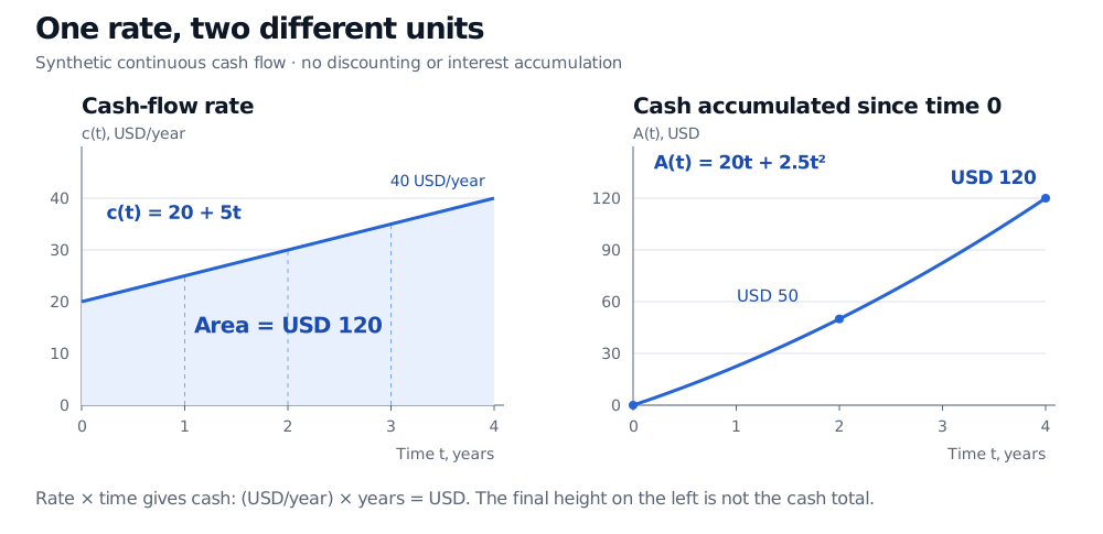
where t is measured in years and c(t) in USD/year. The intercept has units USD/year; the slope has units USD/year². The payment rate starts at USD 20/year and ends at USD 40/year. Ignore interest earned on receipts and add the payments without discounting.
The total cash received is
∫04c(t)dt=[20t+25t2]04=80+40=120 USD.
Here 0 and 4 are the bounds of integration, c(t) is the integrand, and dt specifies time as the integration variable. Writing the variable as u instead would give the same total.
We evaluated the integral with an antiderivative: F(t)=20t+25t2 has derivative c(t). The fundamental theorem of calculus says that, for a continuous integrand, the integral is F(4)−F(0). An arbitrary constant in F cancels between the endpoints. The definite result is USD 120, without an extra +C; the indefinite integral denotes a family of antiderivatives.
Synthetic cash-flow rate rises from USD 20/year to USD 40/year over four years. Shaded rate-times-time area is USD 120. The separate accumulation curve starts at USD 0, reaches USD 50 after two years and USD 120 after four years.
Original synthetic example. The left panel's height measures USD/year; its shaded area and the right panel's height measure USD. Payments are added without discounting or interest accumulation.
A second calculation uses geometry: the area is a rectangle of 20×4=80 USD plus a triangle of 21×4×20=40 USD. Equivalently, this affine rate averages USD 30/year over four years. Multiplying only the final rate by four would incorrectly treat every earlier payment rate as USD 40/year.
What the limiting sum adds
Partition [a,b], with a<b, into small intervals. Choose a sample point ti∗ in each interval of width Δti. For an integrable function,
∫abf(t)dt=maxiΔti→0limi=1∑nf(ti∗)Δti,
with the same limit for every choice of sample points. Continuity on the closed interval is a sufficient condition. Each cash-flow term is a local rate multiplied by a time width, so the sum already has cash units before taking the limit.
For the rising-payment example, equal-width left-endpoint sums underestimate the total, while right-endpoint sums overestimate it:
Equal time intervals
Left-endpoint total, USD
Right-endpoint total, USD
4
110
130
16
117.5
122.5
The exact formulas are Ln=120−40/n and Rn=120+40/n, both approaching USD 120. This is an approximation method that explains the integral's meaning even before finding an antiderivative. More generally, integrals need not have convenient elementary antiderivatives; numerical integration can still approximate them.
Signed accumulation and the direction of the bounds
A definite integral counts contributions below the horizontal axis negatively. If a different synthetic net cash-flow rate is g(t)=20−10t USD/year on the same four-year interval, the first two years contribute USD 20 and the last two contribute −USD 20. Its integral is zero. The total unsigned flow is USD 40, computed by integrating ∣g(t)∣. Net zero does not mean no cash moved, or that there was no interim funding need.
Two useful bookkeeping identities are
∫aaf(t)dt=0,∫baf(t)dt=−∫abf(t)dt.
Thus reversing our original bounds gives −USD 120. This is an orientation convention, not a statement that the contract actually paid negative cash. Adjacent periods also add: the original contract pays USD 50 over years 0–2 and USD 70 over years 2–4, totalling USD 120.
Accumulation is not automatically present value
The USD 120 calculation adds cash paid at different dates. To obtain present value at time zero using specified deterministic discount factors, change the integrand:
PV0=∫04c(t)D(0,t)dt.
The dimensionless factor D(0,t) converts time-t cash to time-zero value. With a constant continuously compounded rate r, it is e−rt, where r and t use consistent year units. Positive r makes this positive stream's present value less than USD 120; when r=0, it equals USD 120. The integral operation does not choose the discount model for you.
For further study, Integration in the Mathematics Primer develops antiderivatives, substitution and a discounted cash-flow example. Its public page is a preview; the full lesson requires membership.
Sources
James Stewart, Single Variable Calculus: Early Transcendentals, sixth edition, Thomson Brooks/Cole, 2008, §§5.2–5.4: definite integrals, the fundamental theorem and net change.