A global minimum is the smallest objective value attained across the whole feasible domain. Separate value from minimiser, prove a cost floor, and check constraints and attainment.
Global minimum
A global minimum is the smallest value an objective function attains over its entire feasible set. If D is that set, a feasible point x∗ is a global minimiser when
f(x∗)≤f(x)for every x∈D.
The minimum is the output f(x∗); the minimiser is the input x∗. An optimisation report should give both. “Minimum cost: USD 4” does not tell a trader which control setting achieves it, while “use setting 3” does not report the objective value.
“Global” refers to all feasible choices in the stated model. It does not claim that the model captures every real trading opportunity, risk or cost. A local minimum only compares a point with nearby feasible choices.
A cost floor you can prove
Suppose a researcher tests a hypothetical one-period hedge policy. Its decision variablex is a continuous, dimensionless, normalized control setting, restricted to 0≤x≤8. A synthetic model assigns the policy a total cost
J(x)=(x2−6x+13)USD.
The polynomial's numerical coefficients are chosen for illustration; they are not fitted execution costs or empirical hedge performance. A lower model cost is preferred. Completing the square gives a certificate covering every possible setting:
J(x)=((x−3)2+4)USD≥4USD.
Equality holds exactly when x=3, which is feasible. Therefore
x∈[0,8]minJ(x)=4USD,x∈[0,8]argminJ(x)={3}.
The notation argmin returns the set of minimisers, even when it contains just one element. Several choices can tie for the same global minimum; “global” does not mean “unique.” Here the square is zero at only one setting, so uniqueness follows too.
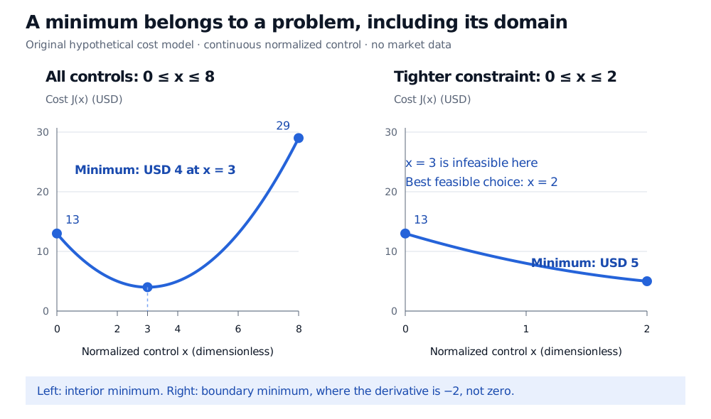
The endpoints cost J(0)=13USD and J(8)=29USD. Comparing these with J(3) agrees with the result. The stronger argument is the nonnegative-square identity: a sampled chart or a search over a few settings alone would not rule out an unseen lower value between samples.
Two charts of the synthetic USD cost J(x). On normalized control interval 0 to 8, the minimum is USD 4 at x equal to 3, and endpoints cost USD 13 and USD 29. Restricting the interval to 0 to 2 moves the minimum to boundary x equal to 2, costing USD 5.
Original hypothetical cost model. Both panels use the same vertical scale; changing the feasible domain changes the best attainable cost.
The constraint is part of the answer
Now impose a tighter constraint: 0≤x≤2. Setting 3 is unavailable. The cost decreases throughout this new interval, so the global minimiser is its right endpoint:
x∗=2,J(2)=5USD.
For a direct check, the difference from that endpoint cost factors as
J(x)−J(2)=(x−2)(x−4)USD≥0,0≤x≤2.
Both factors are nonpositive on this interval. The derivative at the solution is J′(2)=−2USD per unit of normalized control, rather than zero. Moving right would reduce cost, but violates the constraint. A boundary optimum need not have a zero derivative, even when the underlying formula is differentiable there.
For a continuous one-variable function on a closed bounded interval, compare values at both endpoints and every interior critical point, including points where the derivative does not exist. Solving f′(x)=0 only finds some candidates. A stationary point might be a maximum or neither kind of extremum. The closed-interval comparison method is described in OpenStax, §4.3.
Existence, attainment and convexity answer different questions
Does a minimum exist? A continuous real-valued function on a nonempty compact feasible set attains its minimum. In finite-dimensional Euclidean space, compact means closed and bounded. These are sufficient conditions, not a requirement for every problem that has a minimum.
Is a lower bound actually reached? Keep the same cost but allow only 3<x≤8. Every feasible setting costs strictly more than USD 4. Yet xn=3+1/n is feasible for every positive integer n, and
J(xn)=(4+n21)USD⟶4USD.
USD 4 is the infimum, or greatest lower bound, but there is no global minimiser on this domain: setting 3 is excluded. Reporting a minimum of USD 4 would wrongly imply attainability.
Does a local solution certify a global one? For a convex function on a convex feasible set, every local minimiser is global. Strict convexity gives at most one minimiser, while existence still needs an argument. For a differentiable convex objective, the first-order inequality
f(y)≥f(x∗)+∇f(x∗)⊤(y−x∗)
provides a useful certificate: if the final inner product is nonnegative for every feasible y, then x∗ is globally optimal. Zero gradient is one way to satisfy this condition, but the boundary example shows why it is not the only way. See Boyd and Vandenberghe, §4.2.3.
In portfolio construction or calibration, a solver's “converged” message needs to be read against these distinctions: a feasible model, an attained solution, and evidence of global optimality are separate claims. The Constrained and Convex Optimisation lesson develops boundary constraints, convex certificates and minimum-variance portfolios. The public page is a preview; the full lesson requires membership.
Sources
Cornuéjols, G., Peña, J., and Tütüncü, R. Optimization Methods in Finance, 2nd edition, Cambridge University Press, 2018: Chapter 1, §20.3 and Appendix A.2.
Stewart, J. Single Variable Calculus: Early Transcendentals, 6th edition, Thomson Brooks/Cole, 2008: §4.1, “Maximum and Minimum Values.”