A convex function lies below its chords. Compare cost at an average order size with average cost, distinguish strict and strong convexity, and apply the right calculus tests.
Convex function
A convex function assigns a value to an average input that is no greater than the corresponding average of the endpoint values. In one dimension, its graph lies on or below every chord joining two points on the graph. This is why a convex trading-cost model penalises variation in order size, and why a convex objective can make a minimisation problem easier to solve.
Let D⊆Rn be a convex set: for every x,y∈D and λ∈[0,1], the point λx+(1−λ)y also belongs to D. A real-valued function f:D→R is convex if
f(λx+(1−λ)y)≤λf(x)+(1−λ)f(y)for all x,y∈D,λ∈[0,1].
The same weight must appear on each side: λ weights x on the left and f(x) on the right. The domain condition ensures that every input being compared is allowed. For a one-variable function, that domain can be an interval such as [0,∞).
No smoothness is required. A corner in the graph does not prevent convexity. Reversing the inequality defines a concave function; an affine function f(x)=ax+b satisfies equality throughout and is both convex and concave.
A model cost of changing order size
Suppose the total execution cost of an order is modelled as
C(q)=0.01q2,q≥0,
where q is order size in shares and C(q) is in USD. Sizes are treated as continuous for this model. The coefficient has units USD per share squared. This is a hypothetical cost assumption, not an estimate of a particular market's impact or an assertion that actual execution cost is always quadratic.
Order size
Total model cost
100 shares
USD 100
200 shares
USD 400
300 shares
USD 900
The average of 100 and 300 shares is 200 shares, but the two cost calculations differ:
C(2100+300)=400<2C(100)+C(300)=500.
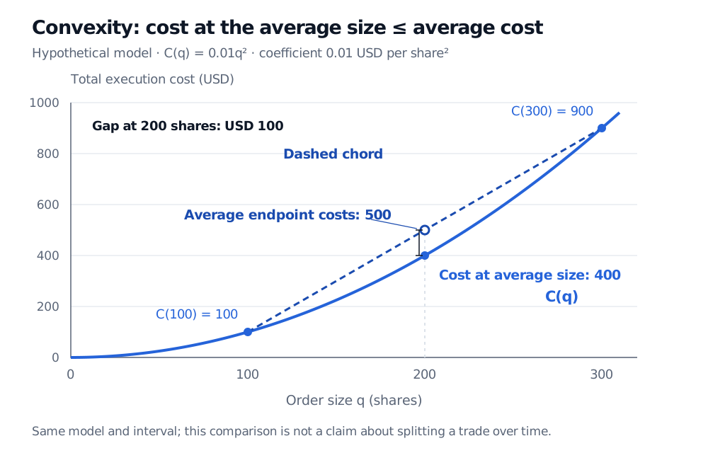
Synthetic total execution cost C(q) = 0.01q squared USD. At 100 and 300 shares, costs are USD 100 and USD 900. At 200 shares, cost is USD 400, while the chord gives the average endpoint cost USD 500: a gap of USD 100.
Original hypothetical cost model. The solid curve gives cost at each size; the dashed chord averages the two endpoint costs. Axes show shares and total USD, rather than average cost per share.
One interpretation is a comparison between a certain 200-share order and a lottery that submits 100 or 300 shares with equal probability under the same cost model. Both have an average size of 200 shares. The certain size costs USD 400; the lottery's expected cost is USD 500. This is the two-outcome form of Jensen's inequality.
It is not yet a trade-splitting result. Executing two orders changes the trading schedule, and may change liquidity, market impact, fixed fees and exposure to price movements. The convexity comparison above evaluates different sizes under one stipulated cost function; it does not establish that the same function applies independently to successive slices.
For this quadratic, the entire definition can be verified algebraically:
λC(x)+(1−λ)C(y)−C(λx+(1−λ)y)=0.01λ(1−λ)(x−y)2≥0.
The gap is positive for distinct sizes and an interior weight, and zero when the sizes coincide or the weight is 0 or 1. Checking one chord illustrates convexity; this identity proves it for every permitted pair and weight.
Convex, strictly convex and strongly convex
Ordinary convexity uses ≤ and allows straight segments. A strictly convex function uses < whenever x=y and 0<λ<1. The cost function above is strictly convex. A straight line is convex but fails this stricter condition.
A strongly convex function has a uniform quadratic amount of curvature. In the Euclidean convention, f is m-strongly convex, for some m>0, when
x⟼f(x)−2m∥x∥22
is convex on its domain. Strong convexity implies strict convexity, which implies convexity. The converse implications fail. For example, f(x)=x4 is strictly convex on R, but its curvature becomes zero at the origin, so it has no positive uniform quadratic curvature bound there. The numerical value of a strong-convexity parameter also depends on the input's units and scaling.
Calculus tests are useful, but they are not the definition
For a differentiable function on an open convex domain, convexity is equivalent to
f(y)≥f(x)+∇f(x)⊤(y−x)for every x,y in the domain.
This says that a tangent line or plane is a global lower bound. Chords lie above the graph; tangents lie below it. For the cost model, the tangent at 200 shares is 400+4(q−200), with slope USD 4 per additional share, and
C(q)−[400+4(q−200)]=0.01(q−200)2≥0.
For a twice continuously differentiable one-variable function on an open interval, convexity is equivalent to a nonnegative second derivative throughout that interval. In several variables, the corresponding test is a positive semidefinite Hessian matrix at every point of an open convex domain. Checking curvature at one point does not establish convexity over the whole domain.
A call option's expiry payoff, max(ST−K,0), is another convex function of its terminal underlying price. Its kink at the strike is allowed. It is not strictly convex: for strike 100, payoffs at terminal prices 110, 120 and 130 are 10, 20 and 30, so the midpoint comparison is equality. This payoff property does not make every option price convex in every pricing input, nor every option strategy convex.
What convexity buys an optimiser
When minimising a convex function over a convex feasible set, every local minimum is a global minimum. If a better feasible point existed, moving a small distance towards it along the feasible segment would already improve the objective, contradicting local minimality.
Strict convexity gives at most one minimiser, not automatic existence. The strictly convex function x2 on the open domain (0,1) approaches zero without attaining it. Convexity also does not require a bowl with a visible bottom: ex is increasing and convex. Finally, integer trade sizes or other nonconvex constraints can break the feasible-segment argument even when the objective itself is convex.
The Constrained and Convex Optimisation lesson develops this result into portfolio constraints and optimality conditions. The public page is a preview; the full lesson requires membership. The broader convex optimisation concept combines the objective's shape with the structure of the feasible set.
Sources
Cornuéjols, G., Peña, J. and Tütüncü, R. Optimization Methods in Finance, 2nd ed., Cambridge University Press, 2018, Appendix A.2, pp. 324–325: convex domains, chord inequality and quadratic functions.
Boyd, S. and Vandenberghe, L. Convex Optimization, Cambridge University Press, 2004, §§3.1.1, 3.1.3–3.1.4 and 9.1.2: strict convexity, derivative characterisations and strong convexity.
Boyd, S. and Vandenberghe, L. Convex functions lecture slides, slides 3–2, 3–3, 3–7 and 3–8: definitions, affine examples, tangent bounds and Hessian tests.