A local minimum beats nearby feasible choices. See why a strict interior trough can still lose to a boundary, and why zero derivatives are only candidates.
Local minimum
A local minimum is a feasible point where an objective function is no larger than at any sufficiently nearby feasible point. It answers a neighborhood question: can a small allowed change improve the objective? A global minimum answers the stronger question across the entire feasible set.
For a quant researcher minimizing a calibration or strategy-selection loss, that distinction matters. A solver can find a genuine local minimum while another admissible parameter choice produces a much lower loss.
What “nearby” allows
Let D be the feasible set. A point x∗∈D is a local minimizer if some radius ε>0 satisfies
f(x∗)≤f(x)for every x∈D with ∣x−x∗∣<ε.
The point x∗ is the minimizer; f(x∗) is the minimum value. “Local minimum” commonly refers to either, with context supplying the distinction.
This non-strict, or weak, definition permits ties. A strict local minimum requires f(x∗)<f(x) at every other feasible point in some neighborhood. Thus a constant objective has weak local minima everywhere, but no strict local minimum on a real interval. Strictness does not mean globally best.
Here neighborhoods are relative to D: infeasible points do not count. An endpoint can therefore be a local minimum even when the unconstrained function continues downhill outside the permitted interval. Some introductory calculus treatments reserve “local extremum” for interior points; the relative-domain convention used here also covers constrained problems.
A research loss with a better answer elsewhere
Suppose a researcher varies a single normalized model parameter x, with allowed range [−3,2], and minimizes the synthetic loss
f(x)=x3−3x.
Both x and the reported loss are dimensionless. Think of x as a parameter's displacement from a fixed reference divided by a fixed positive scale. The loss is an illustrative signed research score, with lower values preferred; it is neither squared error nor an observed trading loss. Negative values are allowed.
At x=1, the loss equals −2. To establish a strict local minimum directly, write a small change as h:
f(1+h)−f(1)=h2(3+h)>0when 0<∣h∣<1.
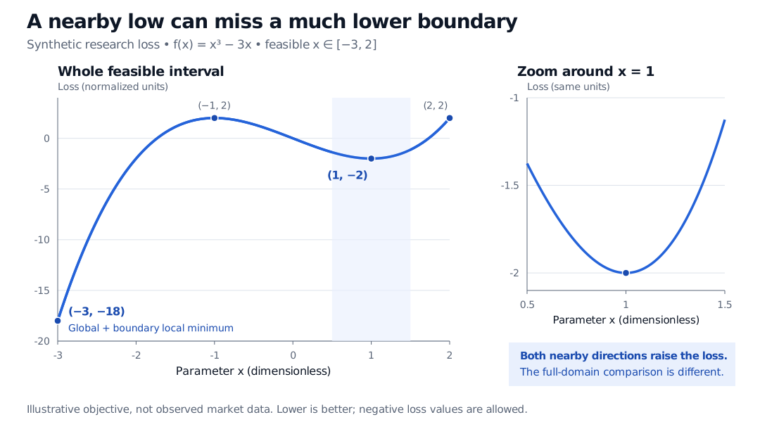
Both small positive and negative changes worsen the loss. All such points remain feasible. But the left boundary gives f(−3)=−18, which is much lower than −2.
Synthetic loss x cubed minus 3x on the dimensionless interval from minus 3 to 2. The interior local minimum at x equals 1 has loss minus 2; the global boundary minimum at x equals minus 3 has loss minus 18. A zoom shows the loss rising on both sides of x equals 1.
Original synthetic objective, with normalized parameter and loss units. The right panel magnifies the shaded interval from 0.5 to 1.5; it is a separate scale view, not a different objective.
The boundary is not merely better than the interior trough: it is globally best on this domain. For every x∈[−3,2],
f(x)+18=(x+3)[(x−23)2+415]≥0.
The bracket is strictly positive, so equality holds only at x=−3. This proves the unique global minimizer. It is also a strict local minimizer relative to the feasible interval. Consequently x=1 is the only interior local minimum here, not the only local minimum under our convention.
A zero derivative gives a candidate
For a differentiable function, an interior local minimum must be a stationary point: f′(x∗)=0. The reverse implication fails. In this example,
f′(x)=3x2−3,f′′(x)=6x.
Both −1 and 1 have zero first derivative. The second derivative separates them: f′′(1)=6>0 establishes a strict local minimum, whereas f′′(−1)=−6<0 establishes a local maximum. The sufficient test assumes twice continuous differentiability near the stationary point, which this polynomial satisfies.
A zero second derivative is inconclusive. At zero, x4 has a strict minimum, while x3 has neither a minimum nor a maximum. Nondifferentiable minima also exist: ∣x∣ is minimized at zero, where its derivative does not exist. The feasible boundary −3 in our example is another reason not to search only for zero derivatives: f′(−3)=24.
Reading an optimizer's result
A small reported gradient is evidence of approximate stationarity, not a certificate of local or global minimality. Check feasibility, the objective in nearby allowed directions, and the relevant curvature conditions. In several variables, inspecting each coordinate separately can miss a descending combined direction; the full Hessian matrix matters.
Different starting points and broader searches can reveal a better solution in a nonconvex problem, but a finite collection of unsuccessful searches does not prove global optimality. A stronger structural result is available when the objective is a convex function on a convex feasible set: every local minimum is global. The cubic above does not meet that condition across its whole feasible interval.
For the multivariable classification and descent-method mechanics, continue to Unconstrained Optimisation. Constrained and Convex Optimisation develops feasible directions, boundary restrictions and the convexity guarantee. Both offer public previews; the full lessons require membership.
Sources
Gérard Cornuéjols, Javier Peña and Reha Tütüncü, Optimization Methods in Finance, second edition (2018), §20.3, “Optimality Conditions”: feasible-neighborhood definitions and first- and second-order tests.