A local maximum is an objective function value that is at least as high as every value at sufficiently nearby feasible inputs. The input achieving it is a local maximiser. A trading-model search can reach such a point and find that every small parameter adjustment makes its score worse, while a distant setting performs better under the same model.
“Nearby” is the qualifier. A global maximum must beat or tie every feasible alternative, however far away.
What counts as nearby?
For a real-valued function on a feasible set , a point is a local maximiser if some radius satisfies
The radius need only exist; the inequality need not hold at every distance. The maximum is strict if every distinct feasible point in that neighbourhood has a strictly lower value. Ordinary, non-strict local maxima allow ties. For a constant objective on , every point is a local maximiser, but none is strict. A local maximum therefore need not look like a pointed hilltop.
This article takes neighbourhoods relative to the feasible set, following the optimisation convention used by Boyd and Vandenberghe, §4.1.1. An endpoint can qualify because only feasible nearby points are compared. Some calculus texts, including OpenStax, reserve “local extremum” for interior points and call endpoint extrema separately. The two conventions describe the same comparisons; they attach different labels at a boundary.
A research parameter that reaches the wrong peak
Suppose a researcher can choose a continuous, dimensionless, normalised parameter . A deliberately synthetic model assigns it the dollar objective
The coefficients are stipulated. This is a hypothetical objective landscape for a parameter search, not an observed return curve, a market calibration or a forecast of trading profits. Negative parameter values are permitted settings, not negative probabilities or portfolio weights.
Its first two derivatives are
The slope is positive on , negative on , and positive on . Thus the curve rises to , falls away, then rises again after the local minimum at . At the interior peak,
The negative second derivative confirms a strict local maximum. There is also a direct neighbourhood check: write . Then
Every distinct setting within that radius scores less than USD 2. Yet the whole-domain comparison gives:
| Setting | Objective , USD | Role |
|---|---|---|
| Left endpoint | ||
| Strict interior local maximum | ||
| Interior local minimum | ||
| Strict global maximum at the right endpoint |
These are all the interior stationary candidates and both endpoints. The derivative signs show there are no omitted higher values between them. Consequently, the global maximum is USD 18 at . Under the relative-domain convention, is also a strict local maximiser: nearby feasible inputs lie to its left and have lower values. The polynomial's derivative there is , which is allowed because the maximiser is on a boundary.
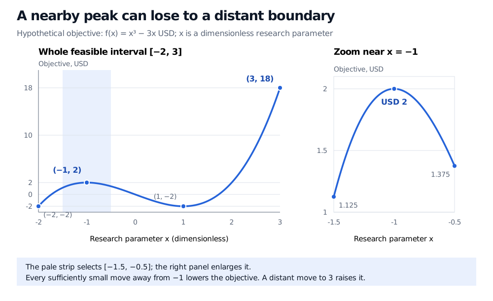
Original hypothetical example. The pale strip selects for the zoom; its endpoint scores are USD 1.125 and USD 1.375. A local comparison certifies that neighbourhood, while global optimality requires the whole feasible interval.
A local search starting near can settle at the lower peak. Trying several starting settings can reveal better candidates, but the best run observed is still not a proof that no better feasible setting exists.
What derivative tests can certify
At a differentiable interior local maximiser, is necessary. It is not sufficient: has derivative zero at 0 and keeps increasing through it. Nor is differentiability required by the definition: has a strict maximum at its corner, where the derivative does not exist.
For a twice continuously differentiable objective near an interior stationary point, is sufficient for a strict local maximum. Zero second derivative is inconclusive; still has a strict maximum at 0. These tests classify local behaviour, not distant alternatives. If software expects a minimisation objective, negate the function: local maxima of become local minima of , and a global maximum becomes a global minimum of .
Additional structure can close the gap. If the objective is concave on a convex feasible set, every local maximiser is global. The cubic example lacks that property over its full interval: its second derivative changes sign. For the extension to several parameters, Unconstrained Optimisation develops stationary points, Hessian classification and ascent methods through utility and calibration examples. Its public preview is available without membership; the full lesson requires membership.
Sources
- James Stewart, Single Variable Calculus: Early Transcendentals, 6th edition, §§4.1 and 4.3 — local versus absolute extrema, first-derivative and second-derivative tests.
- OpenStax, Calculus Volume 1, §4.3, “Maxima and Minima” — interior-point convention, critical candidates and Fermat's theorem.
- Stephen Boyd and Lieven Vandenberghe, Convex Optimization, Cambridge University Press, 2004, §§4.1.1 and 4.2.2 — local optimality among nearby feasible points and the local-to-global property of convex optimisation, applied to maximisation by negating the objective. The cubic example and figure are original.