A global maximum, also called an absolute maximum, is the largest value an objective function actually attains over its entire feasible set. In a portfolio problem, this means no other permitted portfolio scores higher under the stated objective. “Global” describes the scope of that comparison; it does not mean the model has found the best investment in the real world.
For a real-valued function on a nonempty feasible set , a feasible point is a global maximiser when
The maximum value is ; the maximiser is the input . The notation collects all maximising inputs. Ties are allowed: an objective can have several maximisers while having only one maximum value. OpenStax's treatment of absolute extrema makes the whole-domain comparison explicit.
A position-size decision with a certificate
Suppose a deliberately simplified one-period trading model assigns the following net dollar objective to position size:
Here is continuous, dimensionless normalised size, and is measured in USD. The coefficients encode a hypothetical benefit that grows with size and a quadratic size penalty. These are stipulated model inputs, not estimated market returns or a profit forecast; continuous sizing is a divisible-position approximation.
The completed square gives more than a promising candidate:
This inequality holds for every feasible size. Equality holds only at , so
The two endpoints give and USD. Choosing the largest allowed position would therefore produce a worse objective than choosing no position in this model. The best size and the best dollar value answer different questions: 4 is the decision; USD 16 is its objective value.
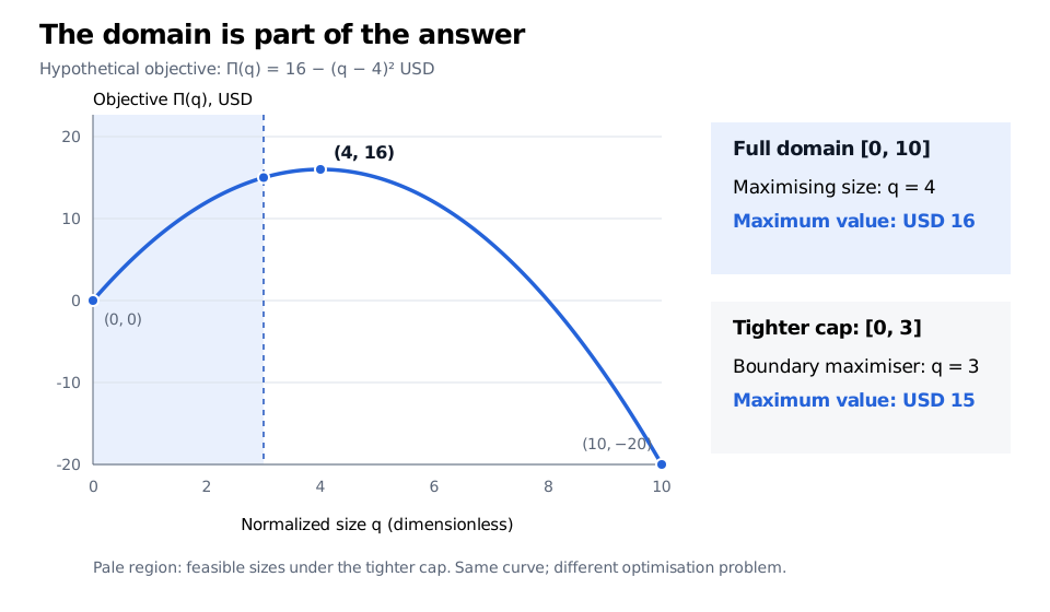
Original hypothetical model. The pale region shows the tighter feasible interval . Changing the feasible set changes the optimisation problem even when the objective curve stays the same.
A stationary point is only one kind of candidate
A local maximum compares nearby feasible inputs. A global maximum must survive comparison with all feasible inputs, including distant alternatives. A local search routine can stop at a nearby peak without certifying that comparison. Checking a finite grid likewise certifies only the points checked unless further structure supplies a bound between them.
In the example, , so the interior maximiser is a stationary point. But stationarity is not a universal requirement. If a tighter position limit changes the feasible set to , then is increasing throughout that interval and its global maximum is USD 15 at the boundary , although . The polynomial's ordinary derivative still exists there; the constraint prevents taking a larger feasible position.
For a continuous one-variable objective on a closed bounded interval, compare the endpoints with every interior candidate where the derivative is zero or fails to exist. This is a complete method when all such candidates have been found and their values can be compared. Smoothness alone does not make an interior stationary point globally best. Useful additional structure includes concavity: on a convex feasible set, any local maximum of a concave objective is global; strict concavity gives at most one maximiser.
For the portfolio version of that reasoning, Constrained and Convex Optimisation develops feasible portfolio weights, bound constraints and conditions that turn local optimality into global optimality. Its public preview is free to read; the full lesson requires membership.
An upper limit need not be attained
Existence comes before searching. The extreme value theorem guarantees that a real-valued continuous function on a nonempty compact feasible set attains a global maximum and minimum. In finite-dimensional Euclidean space, compact means closed and bounded. This guarantees attainment, not uniqueness or an algorithm for finding the answer. Lebl states both the interval theorem and its compact-space extension.
For on , the least upper bound is 1, but no feasible input attains it: every candidate can be improved by . There is no maximum. On the unbounded domain , the same function has no finite upper bound at all. Neither situation should be reported as a successful maximisation.
These are sufficient existence conditions, not necessary ones. For example, attains its global maximum 0 at on the unbounded real line. The domain and objective must be assessed together. A numerical answer becomes a global-optimality claim only when its feasibility, attainment and comparison with the rest of the domain are justified.
Sources
- James Stewart, Single Variable Calculus: Early Transcendentals, 6th edition, §4.1, “Maximum and Minimum Values” — absolute versus local extrema, the extreme value theorem and the closed-interval method.
- OpenStax, Calculus Volume 1, §4.3, “Maxima and Minima” — definitions, endpoint and critical-point candidates, and Fermat's theorem.
- Jiří Lebl, Basic Analysis I: Introduction to Real Analysis, version 5.4, June 2021, Theorems 3.3.2 and 7.5.6 — attainment on closed bounded intervals and compact spaces. The position-size model and figure are original.