Concavity puts a function above its chords. Use a positive-wealth log-utility example to distinguish mean utility from utility of mean wealth, and connect curvature to Jensen’s inequality.
Concavity
Concavity means that a function's value at an average input is at least as large as the corresponding average of its values. Its graph lies on or above every chord between two points on the graph. In finance, this is the shape that makes a stipulated log-utility investor prefer certain wealth to an uncertain outcome with the same mean.
For a real-valued function f on an interval I, the definition is
f(λx+(1−λ)y)≥λf(x)+(1−λ)f(y),x,y∈I,0≤λ≤1.
The left side evaluates the function after averaging the inputs. The right side averages the function values, using the same weights. A chord is the straight segment connecting (x,f(x)) to (y,f(y)); its height at the weighted input is the right side.
Reversing the inequality gives a convex function. Equivalently, f is concave precisely when −f is convex. Strict concavity requires a strict inequality for distinct inputs and an interior weight. A straight line satisfies equality and is both convex and concave.
Two wealth outcomes, two averages
Consider a hypothetical decision-maker whose preferences are represented by expected utility, with
U(W)=ln(WrefW),W>0,Wref=1 USD.
Here W is total terminal wealth. The positive reference wealth makes the logarithm's argument dimensionless; utility itself is dimensionless. This model cannot evaluate zero or negative wealth. Changing the reference adds a constant to utility and leaves the preference comparisons unchanged.
Suppose terminal wealth is USD 100 or USD 400, each with probability one half. These are model outcomes, not observed returns or a forecast.
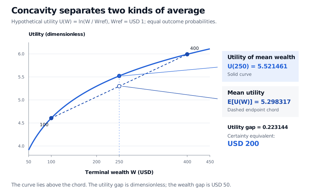
The first number is the utility of receiving USD 250 for certain. The second is the expected utility of the two-outcome lottery. The curve's height at mean wealth exceeds the chord's height there, exactly as concavity predicts.
Hypothetical log utility with reference wealth USD 1. Equal probabilities of wealth USD 100 and USD 400 give mean wealth USD 250. Utility at the mean is 5.521461, above mean utility 5.298317 on the endpoint chord; the certainty equivalent is USD 200.
Original positive-wealth example. The solid log-utility curve lies above its dashed endpoint chord. The utility gap is dimensionless; the certainty-equivalent comparison expresses the effect in USD.
To turn the utility comparison back into wealth, solve U(WCE)=E[U(W)]:
WCE=Wrefexp(E[U(W)])=200 USD.
Under these preferences, the decision-maker is indifferent between the lottery and certain wealth of USD 200. The difference between mean wealth and this certainty equivalent is USD 50. The utility difference, approximately 0.223144, is a different quantity with different units.
This is risk aversion within an expected-utility model. It follows from the assumed increasing, strictly concave utility function. It does not establish that every investor has these preferences, or that a particular investment should be avoided. Nor does the example say USD 50 will be lost: that amount measures the model's valuation of removing this uncertainty.
Curvature is about changing slope
For a twice continuously differentiable function on an open interval, concavity is equivalent to f′′(x)≤0 throughout that interval. In the log example,
U′(W)=W1>0,U′′(W)=−W21<0.
Utility rises with wealth while its marginal increase shrinks. Concavity therefore does not mean that the function must be decreasing. The sign of the first derivative describes increasing or decreasing behaviour; the second derivative describes how the slope changes.
A differentiable concave function lies below each tangent line over the interval, even though it lies above its chords. The distinction matters when replacing a nonlinear utility function with a linear approximation. Concavity also allows corners: f(x)=−∣x∣ is concave on the real line despite having no derivative at zero. The chord definition still applies.
Some calculus texts use concave down for this shape and concave up for convexity. Unqualified “concave” here uses the optimisation convention above. The Curve Sketching lesson develops both directions and inflection points; its public page is a preview and the full lesson requires membership.
From a chord to Jensen's inequality
Jensen's inequality extends the comparison to random inputs:
E[f(X)]≤f(E[X]).
A sufficient setting is a concave real-valued f on an interval containing the possible values of X and its mean, with both E[∣X∣] and E[∣f(X)∣] finite. These conditions hold for the finite positive-wealth example. With strict concavity, a genuinely nonconstant input makes the inequality strict. Ordinary concavity permits equality, including along straight segments.
For log utility, positive wealth alone is not enough to guarantee a finite expected logarithm: outcomes approaching zero can make the downside log terms non-integrable. Check the domain and expectations before exchanging “average utility” for “utility of average wealth.” The Jensen's Inequality and Convexity lesson gives the supporting-line proof and the arithmetic–geometric mean connection. Its public page is a preview; the full lesson requires membership.
Sources
Cornuéjols, G., Peña, J. and Tütüncü, R. Optimization Methods in Finance, 2nd ed., Cambridge University Press, 2018, §10.1, Example 10.2, and Appendix A.2, pp. 324–325: expected-utility portfolio choice and the convex-function framework.
Boyd, S. and Vandenberghe, L. Convex Optimization, Cambridge University Press, 2004, §§3.1.1, 3.1.3–3.1.4 and 3.1.8: concavity, tangent and curvature tests, and Jensen's inequality.
Wolitzky, A. Attitudes toward Risk, MIT 14.121, Fall 2015, slides 2–6: expected utility, concavity, risk aversion and certainty equivalents.