A PSD matrix has nonnegative quadratic forms in every direction. See why covariance can be singular, how zero-risk directions work, and why positive diagonal entries are insufficient.
The important word is semi: a nonzero vector may produce exactly zero. A positive definite matrix instead requires strict positivity for every nonzero vector. Here the real symmetric convention is part of the definition; the complex analogue uses Hermitian matrices and conjugate transpose.
In portfolio risk, PSD is the consistency condition that stops a covariance model from reporting negative variance. It permits duplicate exposures and exact hedges, so a valid covariance need not be invertible.
A hedge that cancels the common shock
Consider two fictional assets with identical one-year simple returns: each returns −15% or +25%, with probability one half for each common outcome. They move together, not independently. Both have mean 5%, standard deviation 20%, and covariance matrix, using decimal returns,
Σ=(0.040.040.040.04).
For signed exposure multipliers w=(w1,w2)⊤, the variance of w1R1+w2R2 is
w⊤Σw=0.04w12+0.08w1w2+0.04w22=0.04(w1+w2)2.
A square cannot be negative, so this proves PSD for every exposure vector at once. Three choices tell the financial story:
Exposure vector
What happens to the common shock
Variance, decimal return squared
(1,−1)⊤
Cancels completely
0
(1,1)⊤
Doubles
0.16
(0.5,0.5)⊤
Remains unchanged
0.04
The first two vectors are exposure combinations, without a fully invested budget restriction. In particular, (1,−1)⊤ sums to zero. The last is a fully invested equal-weight portfolio: holding two copies of the same risk gives no diversification.
The zero direction belongs to the null space: Σ(1,−1)⊤=0. This covariance has rank one and is singular. That is a faithful description of this population, not a failed covariance calculation. The zero-variance spread has zero payoff in this particular example; it supplies no trading profit. More generally, zero variance means a constant model outcome, which must still be compared with prices, funding, costs and trading restrictions before making an arbitrage claim.
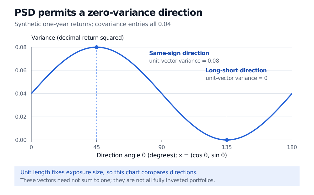
For a synthetic covariance with every entry 0.04, unit exposure vectors have variance 0.08 at 45 degrees and zero at 135 degrees. All directional variances are nonnegative.
Original synthetic one-year example. The chart fixes Euclidean exposure length at one to compare directions; these vectors need not sum to one. Variance is measured in decimal return squared.
Why every covariance passes the PSD test
For a random return vector R with finite second moments and mean μ, its covariance matrix is
Σ=E[(R−μ)(R−μ)⊤].
Consequently, for any fixed vector w,
w⊤Σw=E[(w⊤(R−μ))2]=Var(w⊤R)≥0.
This argument needs no normal-distribution assumption. A zero value means that the corresponding centred return combination is zero almost surely.
The sample version has the same structure. If X contains T>1 aligned observations in rows and centred asset returns in columns, then
Σ=T−1X⊤X,w⊤Σw=T−1∥Xw∥2≥0.
Sample covariance can be singular even without identical assets: its rank is at most min(n,T−1). With at least as many assets as observations, it cannot have full rank. Different pairwise missing-data windows need not yield one common Gram matrix and can produce an indefinite estimate.
Eigenvalues distinguish zero risk from negative risk
Nonnegative eigenvalues make every term nonnegative. Conversely, an eigenvector with a negative eigenvalue immediately produces a negative quadratic form. Our covariance has eigenvalues 0.08 and 0, corresponding to the same-sign and long–short directions. The plotted unit vectors have variance 0.08 and zero there; the unnormalised vector (1,1)⊤ has twice the squared length, hence variance 0.16.
Positive diagonal entries do not establish PSD. Even positive entries throughout are insufficient:
A=(1221),(1,−1)A(1,−1)⊤=−2.
This matrix is symmetric but indefinite, so it cannot be a covariance matrix. For a symmetric two-by-two matrix (ab\bc), the full PSD test is a≥0, c≥0 and ac−b2≥0; looking only at the diagonal misses the covariance restriction.
Using a singular risk model
PSD suffices for a convex portfolio-variance objective. It does not guarantee a unique optimiser or an ordinary matrix inverse. A solver or simulation method should support singular PSD matrices when they are intended: spectral factorisation can retain positive eigenvalues and represent zero directions explicitly. Standard Cholesky routines that require positive definiteness may fail on a valid singular covariance.
In numerical work, judge a small negative computed eigenvalue against matrix scale and the stated tolerance. A materially negative value identifies an invalid covariance estimate; a tiny value near zero may reflect floating-point error. Adding a diagonal adjustment or clipping eigenvalues changes the model and should be an explicit, documented decision.
For the PSD/PD proofs, Gram representation and simulation implications, read Positive Definite Matrices. The full lesson requires membership; a public preview is available. Eigenvalues and Covariance Matrices develops the directional-variance interpretation, with the same access arrangement.
Sources
Sheldon Axler, Linear Algebra Done Right, Second Edition, Chapter 7, “Positive Operators,” Theorem 7.27, pp. 144–146 — nonnegative quadratic forms, eigenvalues and Gram representations.