An eigenvalue is the scalar in Av = λv. See how one yield-shock map amplifies different directions, compute its roots, and separate symmetry from nonnegative risk.
Eigenvalue
An eigenvalue of a square matrixA is a scalar λ for which there is a nonzero vector v satisfying
Av=λv.
The vector is an eigenvector. The eigenvalue tells you how the linear transformation acts along that particular direction: it scales the vector by λ. For a real nonzero eigenvalue, the output stays on the same line; a negative value reverses its orientation. A zero eigenvalue collapses the vector to zero.
The requirement v=0 matters. The zero vector satisfies the equation for every scalar, so allowing it would make the definition useless. Multiplying an eigenvector by a nonzero scalar changes its size but leaves its eigenvalue unchanged. MIT's eigenvalue notes develop this equation and its determinant test.
One map can amplify one shock and preserve another
Suppose a risk analyst deliberately defines the following hypothetical stress transformation for yield changes at two maturity buckets:
(output shock at bucket 1output shock at bucket 2)=A(2112)(input shock at bucket 1input shock at bucket 2).
Both input and output components are measured in basis points (bp). The coefficients of A are dimensionless. This is an assumed scenario rule, rather than an estimated law of yield movements.
Consider two shock patterns:
Input shock, bp
Output shock, bp
Interpretation
(1,1)⊤
(3,3)⊤=3(1,1)⊤
Parallel move is amplified by eigenvalue 3.
(1,−1)⊤
(1,−1)⊤=1(1,−1)⊤
Twist is unchanged by eigenvalue 1.
The eigenvalues are 3 and 1, even though both diagonal entries of the matrix are 2. An eigenvalue generally depends on the whole matrix; it is not a diagonal entry selected by inspection. The diagonal shortcut works for diagonal and triangular matrices.
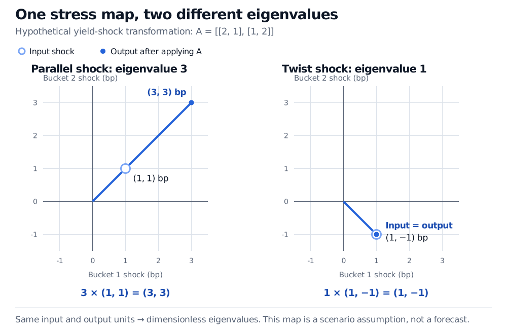
A hypothetical two-bucket yield-shock map with matrix entries 2, 1, 1, 2 sends the parallel input (1, 1) bp to (3, 3) bp, giving eigenvalue 3. It leaves the twist input (1, −1) bp unchanged, giving eigenvalue 1. Both axes measure bucket yield shocks in bp.
Original hypothetical stress map, with equal axis scales. Hollow markers show inputs and solid markers show outputs. The eigenvalues are dimensionless because inputs and outputs share the same units.
These scalars are not expected returns. An eigenvalue of 3 here says that one specified shock pattern becomes three times as large under this map. It does not predict that a bond's price or a portfolio's wealth triples. Converting the output yield shocks into profit or loss requires the book's exposures and a pricing approximation or repricing model.
A generic input need not keep its direction: (1,0)⊤ bp becomes (2,1)⊤ bp. Eigenvalues describe the special patterns that survive the transformation as scalar multiples of themselves.
Finding the scalars without guessing the directions
Rearrange the defining equation as (A−λI)v=0, where I is the identity matrix. A nonzero solution exists exactly when A−λI is singular. Therefore solve the characteristic equation
det(A−λI)=0.
For the stress map,
det(A−λI)=(2−λ)2−1=λ2−4λ+3=(λ−3)(λ−1).
The roots give 3 and 1. Substitution into Av=λv verifies the two directions in the table. Two useful checks agree: the eigenvalues sum to the trace, 3+1=2+2=4, and multiply to the determinant, 3×1=2×2−1×1=3. These identities count repeated eigenvalues with their algebraic multiplicity.
The determinant calculation is useful for small hand examples. For large numerical problems, use an appropriate eigenvalue solver rather than expanding and solving a high-degree characteristic polynomial.
Real, nonnegative and zero mean different things
A real matrix can have complex eigenvalues. For example, the 90-degree rotation
Q=(01−10)
has characteristic equation λ2+1=0, hence eigenvalues i and −i. No nonzero real vector remains on its original line under this rotation. The eigenvalue equation still holds over complex vectors.
A real symmetric matrix has real eigenvalues and an orthonormal eigenbasis, as explained in MIT's symmetric-matrix notes. Symmetry alone does not make the eigenvalues nonnegative. The symmetric matrix diag(1,−1) has eigenvalues 1 and −1.
A covariance matrix has the additional property of being positive semidefinite. For a real eigenvector q of a covariance matrix Σ,
0≤q⊤Σq=λq⊤q⟹λ≥0.
If the observed variables are yield changes in bp, covariance eigenvalues have units bp squared. For a dimensionless eigenvector with Euclidean norm one, λ is the variance of the projected yield change q⊤Δy. That interpretation comes from the covariance model and the normalisation; it does not apply to every matrix called A. The Eigenvalues and Covariance Matrices lesson develops this risk interpretation; the full lesson requires membership, with a public preview available.
A zero eigenvalue means that the square matrix is singular. For a covariance matrix it identifies a direction with zero variance under that model, rather than a guaranteed profitable trade. A materially negative covariance eigenvalue is inconsistent with nonnegative variance; a tiny computed negative value should be assessed against matrix scale and numerical tolerance.
Finally, an n×n matrix has n eigenvalues over the complex numbers, counted with multiplicity. This does not guarantee n independent eigenvectors. Whether an eigenbasis exists determines whether an eigenvalue decomposition is available.
Sources
Gilbert Strang, Introduction to Linear Algebra, 5th edition, Wellesley–Cambridge Press, 2016, §6.1 (eigenvalue equation, characteristic equation, trace, determinant and complex eigenvalues), §6.4 (real symmetric matrices), and §6.5 (positive definite and semidefinite matrices).