Eigenvector: Definition & Examples

An eigenvector of a square matrix

A

is a nonzero vector

\mathbf{v}

that the matrix maps to a scalar multiple of itself:

A\mathbf{v}=\lambda\mathbf{v},\qquad \mathbf{v}\ne\mathbf{0}.

The scalar

\lambda

is the associated eigenvalue. For real vectors and eigenvalues, the image stays on the same line: a positive eigenvalue preserves orientation, a negative one reverses it, and zero sends the vector to zero. Zero is an allowed eigenvalue; the zero vector is never an eigenvector.

For a quant, an especially useful case is a covariance matrix. Its eigenvectors identify combinations of assets that separate the model's return variation into uncorrelated modes. They describe risk directions, not forecasts of which assets will outperform.

Two assets: together or against each other

Suppose a risk analyst uses this hypothetical covariance matrix for two assets' simple returns over the same fixed horizon:

\Sigma=\begin{pmatrix} 0.04&0.01\\ 0.01&0.04 \end{pmatrix}.

Returns are recorded as decimals, so the entries have units of squared decimal return. Each asset has volatility $\sqrt{0.04}=20\%$ over that horizon. Their correlation is $0.01/(0.20\times0.20)=0.25$ .

Multiplying by two candidate directions gives

\begin{aligned} \Sigma\begin{pmatrix}1\\1\end{pmatrix} &=\begin{pmatrix}0.05\\0.05\end{pmatrix} =0.05\begin{pmatrix}1\\1\end{pmatrix},\\ \Sigma\begin{pmatrix}1\\-1\end{pmatrix} &=\begin{pmatrix}0.03\\-0.03\end{pmatrix} =0.03\begin{pmatrix}1\\-1\end{pmatrix}. \end{aligned}

Both are eigenvectors. The first combines the assets with the same sign; the second contrasts them. Positive covariance makes the same-sign direction more variable than the opposing-sign direction when their lengths are matched. By comparison, $(1,0)^\top$ is not an eigenvector: its image $(0.04,0.01)^\top$ acquires a second component and leaves the original line.

These names describe this two-asset model. In a large universe, a leading eigenvector need not mean “the market,” and a low-variance direction need not be a profitable spread.

Why the normalisation changes the risk number

Eigenvectors do not come with a position size. If $\mathbf{v}$ is an eigenvector, then $c\mathbf{v}$ is another for every nonzero scalar $c$ :

A(c\mathbf{v})=cA\mathbf{v}=\lambda(c\mathbf{v}).

In particular, flipping every sign produces an equally valid eigenvector. To compare directions, it is common to set their Euclidean norm to one:

\mathbf{q}_+=\frac{1}{\sqrt{2}}\begin{pmatrix}1\\1\end{pmatrix}, \qquad \mathbf{q}_-=\frac{1}{\sqrt{2}}\begin{pmatrix}1\\-1\end{pmatrix}.

For any unit eigenvector of a covariance matrix,

\text{Var}(\mathbf{q}^\top\mathbf{R}) =\mathbf{q}^\top\Sigma\mathbf{q} =\lambda\mathbf{q}^\top\mathbf{q} =\lambda,

where $\mathbf{R}$ is the return vector. Thus the unit directions above have variances $0.05$ and $0.03$ . Their volatilities are approximately $22.36\%$ and $17.32\%$ over the chosen horizon. These are linear return combinations with unit vector length; their coefficients are not automatically fully invested portfolio weights.

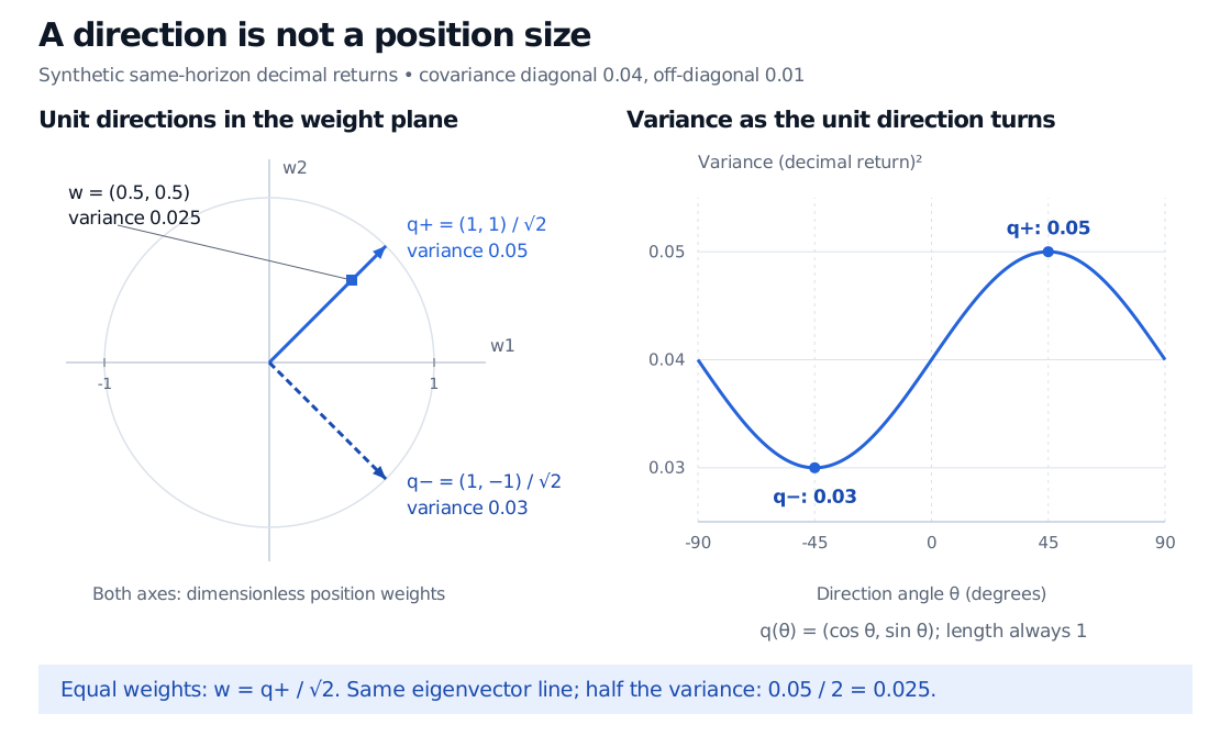
Two unit eigenvectors in a dimensionless weight plane and their directional variance curve. The same-sign unit direction has variance 0.05; the opposite-sign unit direction has variance 0.03. Fully invested weights 0.5, 0.5 share the same-sign line but have variance 0.025.

Original synthetic two-asset example. The curve evaluates variance only for unit-length directions. The square marker in the left panel uses a smaller position on the same eigenvector line.

A fully invested equal-weight portfolio has $\mathbf{w}=(0.5,0.5)^\top=\mathbf{q}_+/\sqrt{2}$ , so

\text{Var}(\mathbf{w}^\top\mathbf{R}) =\frac{1}{4}(0.04+0.01+0.01+0.04) =0.025.

Its volatility is approximately

15.81\%

, not

22.36\%

. The direction is unchanged, but variance scales with the square of position size. Likewise, weights

(0.5,-0.5)^\top

, with gross exposure one, have variance

0.015

; they sum to zero and cannot be turned into weights summing to one simply by dividing by their sum. A tradable portfolio still needs explicit capital, leverage, financing and short-sale conventions.

From two directions to a risk decomposition

A real covariance matrix is symmetric and positive semidefinite. The spectral theorem guarantees an orthonormal basis of eigenvectors

\mathbf{q}_i

with nonnegative eigenvalues

\lambda_i

. For any position vector, define

a_i=\mathbf{q}_i^\top\mathbf{w}

. Then

\mathbf{w}^\top\Sigma\mathbf{w} =\sum_i\lambda_i a_i^2.

This separates a mode's inherent variance, $\lambda_i$ , from the book's exposure to it, $a_i$ . A high-variance mode contributes little to a book that barely loads on it. Conversely, a low-variance spread can become a large risk after leverage.

In principal component analysis, the leading unit eigenvector maximises projected variance. Here it accounts for $0.05/(0.05+0.03)=62.5\%$ of the sum of the two assets' variances. That fraction measures a property of the covariance model; it is not the share of every portfolio's risk and says nothing about expected return. Orthogonal component scores are uncorrelated, which alone does not make them statistically independent.

Reading eigenvectors from data

A few checks matter when interpreting a reported eigenvector:

Sign: a software output may reverse all signs between runs without changing the underlying line. Compare aligned directions rather than individual sign changes.
Repeated eigenvalues: if an eigenvalue is repeated, its eigenspace may have many equally valid orthonormal bases. Even distinct but closely spaced eigenvalues can produce individual directions that move substantially when the estimated covariance changes. A stable subspace can be more meaningful than one labelled vector.
Units and scaling: both coordinates above are same-horizon returns in the same decimal convention. Changing the scale of only one variable generally changes covariance eigenvectors. Using a correlation matrix instead means analysing standardised variables; its coefficients require conversion before being read as exposures to the original returns. Mixing raw currency moves, basis-point changes and returns without a stated scaling convention makes the geometry economically ambiguous.
Matrix type: general square matrices need not have real eigenvectors or a complete eigenvector basis. The covariance conclusions rely on symmetry and positive semidefiniteness. In numerical work, check the residual $\Sigma\mathbf{q}-\lambda\mathbf{q}$ and normalisation, but remember that a small residual does not establish that an estimated risk direction will remain stable out of sample.

For a worked continuation, Eigenvalues and Covariance Matrices develops the spectral decomposition and variance coordinates. PCA and Factor Compression connects those directions to a centred return panel. Both offer public previews; full lessons require membership.

Sources

Gene H. Golub and Charles F. Van Loan, Matrix Computations, 4th edition, Johns Hopkins University Press, 2013, §2.1.7, §7.1.1 and §8.1.3: eigenpairs, symmetric matrices, directional quadratic forms, invariant subspaces and eigenvector sensitivity.
Gilbert Strang, Lecture 4: Eigenvalues and Eigenvectors, MIT OpenCourseWare, 18.065, Spring 2018: real and complex eigenvectors, zero eigenvalues and the symmetric case.
NIST/SEMATECH, e-Handbook of Statistical Methods, §6.5.5.1: Properties of Principal Components: unit-length coefficients, maximum projected variance and diagonal component covariance.

Two assets: together or against each other

Why the normalisation changes the risk number

From two directions to a risk decomposition

Reading eigenvectors from data

Sources

Related terms

Basis

Eigenvalue

Euclidean norm

Matrix

Positive semidefinite matrix

Vector