Euclidean norm: Definition & Examples

The Euclidean norm, or L2 norm, is the non-negative length of a vector: square its coordinates, add them, and take the square root. For a real vector

\mathbf{x}=(x_1,\ldots,x_n)

\lVert\mathbf{x}\rVert_2 =\sqrt{\sum_{i=1}^{n}x_i^2} =\sqrt{\mathbf{x}^{\mathsf T}\mathbf{x}}.

The last expression uses the dot product. In ordinary Cartesian coordinates, this is Pythagoras' theorem extended to any finite number of dimensions. The subscript

2

identifies the norm; it does not mean “square the answer”.

For a quant, this gives a way to measure the size of a pricing-error vector, penalise large coefficients or calculate distance between comparable observations. Its financial meaning comes from what the coordinates represent and how they are scaled.

A length keeps units; a squared length does not

Suppose a model has two pricing residuals of USD 3 and USD 4 per underlying unit, each measured as model price minus observed price. With equal weight on the two residuals,

\lVert(3,4)\rVert_2=\sqrt{9+16}=5.

The root-sum-square error is USD 5 per underlying unit. The squared norm is

25

, with squared-price units. Neither number is the total cash error across a position: that would also require contract quantities and a decision about how signed errors should combine. Squaring removes each residual's sign, so opposite pricing errors do not cancel in this measure.

The squared norm is the sum-of-squares objective in least squares. Minimising a non-negative norm or its square gives the same minimisers, because squaring preserves their order. But the two objectives have different derivatives, scaling and units. A penalty on squared norm is therefore a different numerical object from a penalty on norm.

One sleeve, three different exposure summaries

Consider a hypothetical risky-asset sleeve with signed holdings divided by portfolio net asset value:

\mathbf{w}=(0.6,-0.8).

The first asset is long 60% of NAV and the second short 80%. These are the two risky holdings, not a complete budget vector; cash of 120% of NAV would make the full weights sum to one. For this sleeve:

Measure	Calculation	Value	What it measures
Euclidean norm	$\sqrt{0.6^2+(-0.8)^2}$	$1$	Root-sum-square of risky weights
Gross exposure	$\lvert0.6\rvert+\lvert-0.8\rvert$	$1.4$	Total absolute risky holdings: 140% of NAV
Net exposure	$0.6-0.8$	$-0.2$	Signed risky holdings: −20% of NAV

A unit-length vector can therefore have gross exposure above one and negative net exposure. Normalising a vector to length one does not create a fully invested or market-neutral portfolio.

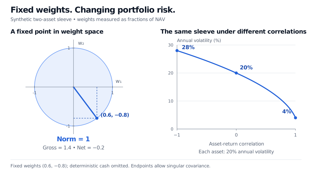
Fixed risky-asset weights 0.6 and minus 0.8 lie on the unit circle, with Euclidean norm 1, gross exposure 1.4 and net exposure minus 0.2. With both assets at 20% annual volatility, portfolio volatility is 28%, 20% and 4% at correlations minus 1, 0 and 1.

Original synthetic example. The same risky weights are held fixed throughout; each asset has 20% annual return volatility. Deterministic cash contributes no variance. Perfect-correlation endpoints allow singular covariance matrices.

Why length is not portfolio volatility

Portfolio volatility depends on the covariance matrix

\Sigma

of asset returns:

\sigma_p=\sqrt{\mathbf{w}^{\mathsf T}\Sigma\mathbf{w}}.

For this sleeve, suppose both assets have annual return standard deviation $\sigma=0.20$ and correlation $\rho$ . Then

\sigma_p =0.20\sqrt{0.6^2+(-0.8)^2+2\rho(0.6)(-0.8)} =0.20\sqrt{1-0.96\rho}.

At correlations

-1

0

and

1

, portfolio volatility is respectively 28%, 20% and 4%, while the weight norm remains exactly one. Positive correlation helps this particular long–short sleeve because the two signed exposures partly offset common movements. These are model comparisons, not estimated market relationships; shorting costs and changing weights are excluded.

Only in the special case

\Sigma=\sigma^2 I

, with equal asset volatilities and zero pairwise covariances, is portfolio volatility simply

\sigma\lVert\mathbf{w}\rVert_2

. More generally, if

\Sigma=B^{\mathsf T}B

, then

\sigma_p=\lVert B\mathbf{w}\rVert_2

: risk is the Euclidean length after a covariance-based transformation. A singular covariance can assign zero volatility to a nonzero holding vector, so that risk measure is then a seminorm on holdings rather than a norm.

Scaling is part of the question

Euclidean geometry requires compatible coordinates. Adding a squared stock price in dollars to a squared yield in basis points has no coherent raw-unit interpretation. Even changing a price quotation from dollars to cents would alter that raw distance and any resulting ranking.

A stated scale $s_i>0$ for each feature gives dimensionless coordinates $z_i=x_i/s_i$ and the explicit measure

\lVert\mathbf{z}\rVert_2=\sqrt{\sum_i\left(\frac{x_i}{s_i}\right)^2}.

Scales might represent measurement uncertainty, a training-sample standard deviation or a chosen economic tolerance. Each answers a different question. Standardising individual features does not by itself remove correlations, and a convenient numerical scaling does not automatically produce a portfolio-risk measure.

There is a related coordinate caveat: an orthogonal matrix preserves Euclidean length, $\lVert Q\mathbf{x}\rVert_2=\lVert\mathbf{x}\rVert_2$ when $Q^{\mathsf T}Q=I$ . Arbitrary rescalings or coordinates in an oblique basis need not preserve the sum-of-squares formula for the original physical length.

Operations that follow from length

For compatible real vectors, the norm is zero exactly at the zero vector, obeys $\lVert a\mathbf{x}\rVert_2=\lvert a\rvert\lVert\mathbf{x}\rVert_2$ , and satisfies the triangle inequality:

\lVert\mathbf{x}+\mathbf{y}\rVert_2 \leq\lVert\mathbf{x}\rVert_2+\lVert\mathbf{y}\rVert_2.

Distance between two vectors is the norm of their difference, $\lVert\mathbf{x}-\mathbf{y}\rVert_2$ . A nonzero vector can be converted to a unit vector by dividing by its norm; $(3,4)/5=(0.6,0.8)$ , for example. The zero vector cannot be normalised this way.

For a time series of

n

comparable observations, root-mean-square is

\lVert\mathbf{x}\rVert_2/\sqrt n

. A sample standard deviation instead centres the observations first and, with the usual

n-1

convention for

n>1

, divides the centred norm by

\sqrt{n-1}

. Raw vector length alone supplies neither that centring nor the statistical denominator.

To develop the geometry, see The Dot Product, Length, and Angle, especially its Length section and triangle-inequality proof. For the risk transformation, Eigenvalues and Covariance Matrices explains how covariance eigenvalues weight squared exposures. Both provide public previews; full lessons require membership.

Sources

Stephen Boyd and Lieven Vandenberghe, Introduction to Applied Linear Algebra: Vectors, Matrices, and Least Squares, §§3.1–3.3 and §17.1: vector norm, distance, standard deviation and portfolio weights.
Lieven Vandenberghe, UCLA ECE133A, “Norm, distance, angle”, Fall 2025, slides 2.2–2.9: norm properties, RMS and de-meaning.
Stanford Convex Optimization Group, “Portfolio optimization”: signed allocation weights, absolute exposure and covariance-based variance.

A length keeps units; a squared length does not

One sleeve, three different exposure summaries

Why length is not portfolio volatility

Scaling is part of the question

Operations that follow from length

Sources

Related terms

Dot product

Least squares

Standard deviation

Vector

Volatility