Eigenvalue decomposition: Definition & Examples

Eigenvalue decomposition, or eigendecomposition, expresses a square matrix through its eigenvectors and eigenvalues. When a matrix

A

has enough independent eigenvectors to form a basis, the decomposition is

A=P\Lambda P^{-1}.

The columns of $P$ are eigenvectors, and the matching eigenvalues sit on the diagonal of $\Lambda$ . It is the same operation described in coordinates where each component is scaled separately. For a quant, that can turn a coupled linear model into separate modes or turn correlated asset returns into uncorrelated risk factors.

The qualification enough independent eigenvectors is essential. A square matrix need not admit this decomposition. The especially useful orthogonal form for real symmetric matrices has a stronger guarantee.

What the three matrices do

Let

P=[\mathbf{v}_1\ \cdots\ \mathbf{v}_n]

and

A\mathbf{v}_i=\lambda_i\mathbf{v}_i

. Column by column, these eigenvalue equations give

AP=P\Lambda

. If the vectors are linearly independent,

P

is invertible, giving the displayed factorisation.

Read the product from right to left:

$P^{-1}\mathbf{x}$ expresses the input in the eigenvector basis.
The diagonal matrix $\Lambda$ scales each eigen-coordinate by its own eigenvalue.
$P$ converts the result back to the original coordinates.

This is a change of basis, so the matrix entries change while the underlying linear operation stays the same. Keep the ordering consistent: the $i$ th column of $P$ must match the $i$ th diagonal entry of $\Lambda$ . Eigenvectors can be rescaled by any nonzero constant, so the displayed factors are not unique.

The symmetric case: perpendicular modes

For a real symmetric matrix,

A=A^\top

, the spectral theorem guarantees a complete orthonormal eigenbasis. We can write

A=Q\Lambda Q^\top, \qquad Q^\top Q=I, \qquad A=\sum_{i=1}^{n}\lambda_i\mathbf{q}_i\mathbf{q}_i^\top.

Here the columns of the orthogonal matrix $Q$ have unit length and are mutually perpendicular, so $Q^{-1}=Q^\top$ . Each term in the sum projects onto one eigen-direction and then scales that projection. A general eigenvector matrix $P$ need not be orthogonal: replacing $P^{-1}$ with $P^\top$ would usually give the wrong answer. Strang's §§6.2 and 6.4 develop these two cases separately.

Symmetry guarantees real eigenvalues. It does not guarantee positive eigenvalues;

\operatorname{diag}(-1,1)

is symmetric too. Covariance matrices have nonnegative eigenvalues because they are positive semidefinite, an additional property.

A model that amplifies common movement

Imagine a synthetic, dimensionless two-signal stress model. One update maps a signal vector to $A\mathbf{x}$ , where

A=\begin{pmatrix}2&1\\1&2\end{pmatrix},\qquad Q=\frac1{\sqrt2}\begin{pmatrix}1&1\\1&-1\end{pmatrix},\qquad \Lambda=\begin{pmatrix}3&0\\0&1\end{pmatrix}.

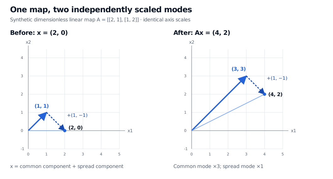
The common-movement direction $(1,1)^\top$ is multiplied by $3$ , while the spread direction $(1,-1)^\top$ is multiplied by $1$ . Direct multiplication verifies $A\mathbf{q}_1=3\mathbf{q}_1$ , $A\mathbf{q}_2=\mathbf{q}_2$ and $A=Q\Lambda Q^\top$ .

Start with $\mathbf{x}_0=(2,0)^\top$ . Its decomposition is particularly transparent:

\mathbf{x}_0=\begin{pmatrix}1\\1\end{pmatrix} +\begin{pmatrix}1\\-1\end{pmatrix}, \qquad A\mathbf{x}_0=3\begin{pmatrix}1\\1\end{pmatrix} +\begin{pmatrix}1\\-1\end{pmatrix} =\begin{pmatrix}4\\2\end{pmatrix}.

Dimensionless synthetic map A with diagonal entries 2 and off-diagonal entries 1. Input (2,0) is the sum of (1,1) and (1,-1). Output (4,2) is the sum of (3,3) and (1,-1): common movement triples and the spread is unchanged.

Original synthetic signal example, with identical dimensionless coordinate scales in both panels. The dashed arrow is the spread component translated to the tip of the common component.

For repeated updates, the adjacent factors $Q^\top Q$ cancel:

A^k=Q\Lambda^kQ^\top,\qquad \mathbf{x}_k=\begin{pmatrix}3^k+1\\3^k-1\end{pmatrix} \quad(k=0,1,2,\ldots).

Updates $k$	First signal	Second signal
0	2	0
1	4	2
2	10	8
3	28	26

In particular,

A^3=Q\begin{pmatrix}27&0\\0&1\end{pmatrix}Q^\top =\begin{pmatrix}14&13\\13&14\end{pmatrix}.

The gap between the signals stays at $2$ , while their common level grows. That conclusion follows from this deliberately specified update rule; it is not an estimated market forecast. A starting vector entirely along the spread direction would have no growing common component.

Covariance uses the same algebra, with a different meaning

Now consider a separate hypothetical risk model for two assets' daily decimal returns:

\Sigma=10^{-4}\begin{pmatrix}2&1\\1&2\end{pmatrix}.

Its eigenvectors are the same $Q$ , but its eigenvalues are $3\times10^{-4}$ and $10^{-4}$ , measured in squared daily-return units. For centred returns $\mathbf{r}$ , the factors $\mathbf{f}=Q^\top\mathbf{r}$ have covariance matrix

\text{Cov}(\mathbf{f})=Q^\top\Sigma Q =\operatorname{diag}(3\times10^{-4},10^{-4}).

The factors are uncorrelated. Independence does not follow without further distributional assumptions. The common direction accounts for $3/(3+1)=75\%$ of total asset variance, which is the interpretation used in covariance-based principal component analysis. This percentage describes variance, not expected return or predictive value.

For fixed portfolio weights $\mathbf{w}$ , write $\mathbf{b}=Q^\top\mathbf{w}$ . Then

\text{Var}(\mathbf{w}^\top\mathbf{r}) =\sum_i\lambda_i b_i^2.

An equal-weight holding,

\mathbf{w}=(1/2,1/2)^\top

, has exposures

b_1=1/\sqrt2

and

b_2=0

. Its daily variance is

1.5\times10^{-4}

and daily volatility is approximately

1.225\%

. All its variance comes from the common factor, despite that factor explaining only

75\%

of the asset universe's total variance. Factor size and a particular portfolio's factor exposure answer different questions.

Do not interpret $\Sigma^3$ as a three-day covariance forecast. Matrix multiplication would cube the squared-return units. Aggregating risk across days instead requires a temporal model, including assumptions about serial dependence.

Where the decomposition can mislead

A repeated eigenvalue does not automatically prevent diagonalisation. The identity matrix has repeated eigenvalues and every basis works. But

J=\begin{pmatrix}1&1\\0&1\end{pmatrix}

has only one independent eigenvector direction: $(J-I)\mathbf{x}=0$ forces $x_2=0$ . It cannot be written $P\Lambda P^{-1}$ , even allowing complex coordinates. A real matrix can also have complex eigenpairs, so real diagonalisation requires a real eigenbasis. The singular value decomposition has broader existence guarantees and applies to rectangular matrices too.

Zero eigenvalues are compatible with diagonalisation; they prevent an ordinary inverse. Repeated eigenvalues permit different orthonormal bases within the same eigenspace. Even with distinct eigenvalues, each eigenvector's sign is arbitrary. In estimated risk models, nearly equal eigenvalues can make individual factor directions sensitive to small data changes. A successful factorisation establishes an algebraic representation, not the reliability or economic meaning of the estimated factors.

For a fuller risk treatment, The Spectral Theorem for Real Symmetric Matrices develops portfolio variance by factor. PCA and Factor Compression connects covariance eigenpairs to a centred returns panel and the cost of discarding modes. Both offer public previews; full lessons require membership.

Sources

Gilbert Strang, Introduction to Linear Algebra, 5th edition, §§6.2, “Diagonalizing a Matrix”; 6.4, “Symmetric Matrices”; and 12.2, “Covariance Matrices and Joint Probabilities.”
Gilbert Strang, Lecture 4: Eigenvalues and Eigenvectors, MIT OpenCourseWare, 18.065, Spring 2018.

What the three matrices do

The symmetric case: perpendicular modes

A model that amplifies common movement

Covariance uses the same algebra, with a different meaning

Where the decomposition can mislead

Sources

Related terms

Basis

Diagonal matrix

Eigenvalue

Eigenvector

Linear independence