Diagonal matrix: Definition & Examples

A diagonal matrix is a square matrix whose entries away from the main diagonal are all zero. Multiplying a vector by it scales each coordinate separately: no input coordinate feeds into another output coordinate. In finance, this describes operations such as assigning a separate volatility scale to each standardised shock.

Write an $n\times n$ diagonal matrix as

D=\operatorname{diag}(d_1,\ldots,d_n), \qquad D_{ij}=0\quad\text{when }i\ne j.

The main diagonal runs from top left to bottom right. Diagonal entries may themselves be zero. The zero matrix and the identity matrix are both diagonal; diagonal does not mean invertible, positive or equal along the diagonal.

Scaling shocks without mixing them

For a column vector, matrix multiplication reduces to

D\mathbf{x}= \begin{pmatrix} d_1x_1\\ \vdots\\ d_nx_n \end{pmatrix}.

A positive entry stretches or shrinks its coordinate, a negative entry also reverses its sign, and a zero entry erases it. The coordinate axes remain invariant, although a vector pointing between the axes can change direction when their scale factors differ.

Consider a hypothetical two-asset return model at one fixed horizon. Let

\mathbf{z}

contain mean-zero, unit-variance, uncorrelated shocks, and define centred decimal returns by

\mathbf{R}=D_\sigma\mathbf{z}, \qquad D_\sigma= \begin{pmatrix}0.20&0\\0&0.10\end{pmatrix}.

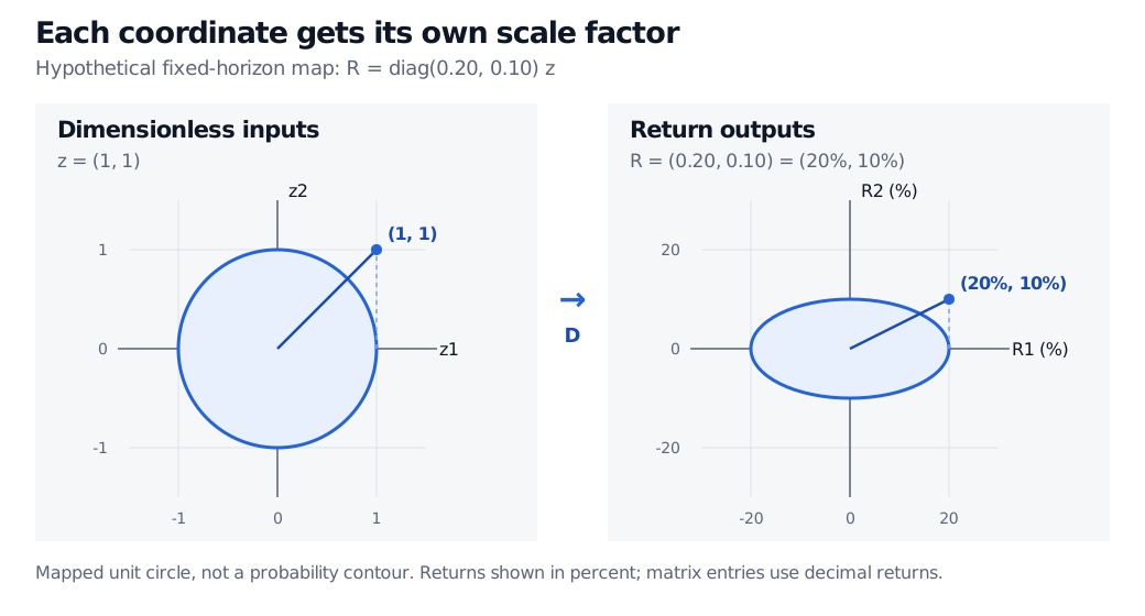
A shock vector

(1,1)^\top

maps to

(0.20,0.10)^\top

: returns of 20% and 10%. The first return depends only on the first shock, and the second only on the second. Here the shocks are dimensionless; the matrix converts them to decimal returns. This is a synthetic illustration, not an estimated market model.

A diagonal map turns a unit circle of dimensionless shocks into an ellipse with return semiaxes 20% and 10%. The input vector (1,1) maps to decimal returns (0.20,0.10), shown as (20%,10%). Each output depends only on its matching input.

Original hypothetical fixed-horizon map. The blue curve is the image of a unit circle, not a probability or confidence contour. Output axes display percent; the matrix uses decimal returns.

The diagonal matrix is the scaling operation. The assumption about the shocks supplies their statistical relationship. Diagonal scaling alone would not remove dependence or covariance already present in the inputs.

A diagonal covariance makes the risk sum separable

In this model the covariance matrix is

\Sigma=D_\sigma I D_\sigma^\top =\begin{pmatrix}0.04&0\\0&0.01\end{pmatrix}.

Notice the distinction: $D_\sigma$ contains volatilities; $\Sigma$ contains variances. Its entries are in squared decimal-return units at the same horizon. Putting 20 and 10 into this formula would mix percentage notation with decimal notation.

For portfolio weights

\mathbf{w}=(0.5,0.5)^\top

, portfolio variance becomes

\begin{aligned} \text{Var}(R_p)&=\mathbf{w}^\top\Sigma\mathbf{w}\\ &=(0.5)^2(0.04)+(0.5)^2(0.01)\\ &=0.0100+0.0025=0.0125. \end{aligned}

The volatility is therefore

\sqrt{0.0125}=0.111803\ldots

, or 11.18% at that horizon. It is not the weighted-average volatility of 15%. The first asset contributes 80% of this portfolio's variance despite having only half its capital weight.

For any diagonal covariance, the same simplification is

\mathbf{w}^\top\Sigma\mathbf{w} =\sum_{i=1}^{n}w_i^2\sigma_i^2.

There are no covariance cross terms. This is a useful model assumption or a property of suitably chosen coordinates, not a general property of asset returns. Replacing an empirical covariance matrix with its diagonal deliberately discards the off-diagonal information. With long-only weights, omitted positive covariances would understate variance; omitted negative covariances would overstate it, holding the diagonal fixed.

Uncorrelated does not generally mean independent. Zero off-diagonal covariance records the absence of linear co-movement, while nonlinear dependence can remain. MIT's covariance notes give a counterexample. A diagonal covariance is enough for the variance calculation above; it is not enough to justify multiplying marginal probabilities when estimating joint losses.

What becomes easy—and what a zero prevents

For two diagonal matrices of the same size, addition and multiplication act on matching diagonal entries. In particular,

\operatorname{diag}(d_1,\ldots,d_n) \operatorname{diag}(e_1,\ldots,e_n) =\operatorname{diag}(d_1e_1,\ldots,d_ne_n).

An inverse matrix exists if and only if every diagonal entry is nonzero. Then

D^{-1}=\operatorname{diag}(1/d_1,\ldots,1/d_n).

For the shock-scaling matrix, the inverse is

\operatorname{diag}(5,10)

: divide each return by its own volatility to recover the shock. If a diagonal entry were zero, every value of that input coordinate would give the same zero output coordinate, so no inverse could recover the lost information. A very small nonzero entry permits an algebraic inverse but amplifies errors when you divide by it. MIT's linear-algebra notes state the precise invertibility condition.

Diagonality also depends on the chosen basis. A matrix that mixes coordinates in the original basis may become diagonal after a valid eigenvalue decomposition. Every real symmetric covariance matrix admits an orthonormal eigenbasis in which its covariance is diagonal. The new coordinates are combinations of assets; those diagonal entries describe their variances, not necessarily the original assets' variances. Changing basis preserves the underlying risk calculation when the portfolio coordinates are transformed consistently.

For the scalar variance calculation and the distinction between covariance and independence, Expectation, Variance and Covariance is available in full with a free signed-in account. Eigenvalues and Covariance Matrices develops the eigenbasis risk sum; its full lesson requires membership, with a public preview.

Sources

Gilbert Strang, Introduction to Linear Algebra, 5th edition (2016), §2.5, Note 6, on diagonal inverses; §12.2 on covariance matrices and the variance of a linear combination. The return model, calculations and figure here are original.
Clark Barwick, MIT 18.06, “Inverting matrices,” 22 February 2016, slide 22 — diagonal invertibility and reciprocal diagonal entries.
Jeremy Orloff and Jonathan Bloom, MIT 18.05, “Covariance and Correlation,” Spring 2022, §2.1 and Example 2 — covariance properties and why zero covariance does not imply independence.

Scaling shocks without mixing them

A diagonal covariance makes the risk sum separable

What becomes easy—and what a zero prevents

Sources

Related terms

Basis

Eigenvalue decomposition

Identity matrix

Matrix

Matrix inverse

Portfolio variance

Vector

Volatility