A linear transformation preserves addition and scaling. Follow a holdings-to-factor-exposure map, interpret its matrix columns and units, and distinguish affine offsets and nonlinear risk.
Linear transformation
A linear transformation, or linear map, is a rule between vector spaces that preserves addition and scalar multiplication. Combining two inputs and then applying the rule gives the same result as transforming each input and combining the outputs. On a risk desk, this lets instrument holdings become a vector of factor exposures: two books can be aggregated before or after their exposures are calculated, provided both use the same fixed loadings.
For a real linear map T:V→W, the requirements are
T(u+v)=T(u)+T(v),T(cu)=cT(u)
for every input pair and every real scalar c, including zero and negative values. These properties are called additivity and homogeneity. Together they imply that T preserves any linear combination:
T(au+bv)=aT(u)+bT(v).
A quick necessary check is T(0)=0. It is not sufficient: squaring a scalar sends zero to zero but fails homogeneity because (2q)2=4q2, rather than 2q2. A few successful numerical tests cannot establish the universal identity; one failed test can refute it.
Turning holdings into exposures
Consider two fictional instruments, A and B, and two return factors. At one market snapshot, their fixed sensitivity matrix is
B=(100.52),e=T(x)=Bx.
Columns are instruments A, B; rows are factors 1, 2. The input x=(x1,x2)⊤ gives signed holdings in lots. The output e=(e1,e2)⊤ gives sensitivities in thousand USD per percentage-point move, abbreviated kUSD/pp. Each matrix entry therefore has units kUSD/(pp·lot). Here one pp means a factor return change from, for example, 0% to 1%, rather than a decimal return of 1.
Fixed sensitivity per lot
Instrument A
Instrument B
Factor 1, kUSD/(pp·lot)
1
0.5
Factor 2, kUSD/(pp·lot)
0
2
Holding two lots of A and three lots of B produces
B(23)=(1(2)+0.5(3)0(2)+2(3))=(3.56)kUSD/pp.
The row calculation adds contributions to the same factor sensitivity, in compatible units. The column calculation tells the portfolio story:
2(10)+3(0.52)=(20)+(1.56)=(3.56).
Thus the two single-instrument books have exposure vectors (2,0) and (1.5,6); adding the books produces their sum. Doubling the holdings to (4,6) doubles exposures to (7,12). Reversing all holdings gives (−3.5,−6), and an empty book gives (0,0). These illustrate the rule. The proof for arbitrary inputs comes from matrix distributivity:
B(au+bv)=aBu+bBv.
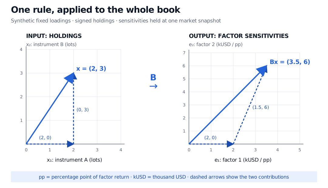
A synthetic fixed loading map sends holdings of 2 lots of A and 3 lots of B to factor sensitivities of 3.5 and 6 thousand USD per percentage point. Dashed contribution arrows show holdings (2,0) and (0,3) becoming exposures (2,0) and (1.5,6), which add to the blue total.
Original synthetic example. The left axes measure holdings in lots; the right axes measure factor sensitivities in kUSD/pp. Arrow lengths across the two panels are not a measure of economic risk.
This map aggregates sensitivities, not realised profit. With factor changes measured in pp, the first-order P&L estimate is ΔV≈e1Δf1+e2Δf2 in kUSD. Fixed position sensitivities add exactly under the model; using them to estimate P&L over a finite market move is a local approximation. Option curvature, changing sensitivities and omitted factors can make that approximation inaccurate.
Why the columns determine the rule
Every fixed m×nmatrix defines a linear map from Rn to Rm. Conversely, once input and output bases are chosen, every linear map between finite-dimensional spaces has a matrix representation. Column j records the output coordinates obtained from input basis vector j. All other outputs follow by linear combination.
A map need not be square or invertible. Several instruments might map to fewer reported factors, and a nonzero holding vector in the null space produces zero of those measured exposures. That alone says nothing about its cost, unmeasured risks or whether it is an arbitrage. A projection can discard a direction; the zero map discards all directions and is still linear.
The input and output also need not describe the same kind of object. Our B converts instrument holdings into factor sensitivities. A change of basis, by contrast, changes coordinates for the same underlying vector. Identical matrix notation does not make those interpretations interchangeable.
Where linearity stops
An affine rule F(x)=Bx+b includes a fixed offset. If b=0, then F(0)=b and the map is not linear: adding two separately transformed books counts the offset twice. For example, a report of existing book exposure plus trade exposure is affine in the new trade holdings. Subtracting the fixed existing exposure leaves a linear map of the trade increment.
A linear exposure map does not make every downstream calculation linear. A quadratic position cost scales by four when a position doubles. With a fixed covariance matrix, portfolio variance is quadratic in holdings; volatility scales by the absolute leverage factor, so reversing a book does not negate its volatility. Neither is a linear map of signed holdings. Execution prices that depend on trade size can also invalidate fixed-coefficient cost calculations.
Finally, linearity is a property of the rule on a vector space. Long-only, integer-lot or budget constraints can restrict admissible portfolios without changing the algebraic exposure rule. The feasible holdings themselves may fail to form a vector space. Keep the model, its permitted inputs and its economic interpretation separate.
Gilbert Strang, Introduction to Linear Algebra, 5th edition (2016), §§8.1–8.2: linearity, affine shifts and matrix representations. The financial example and figure above are original.