A quadratic form is a homogeneous polynomial of degree two: every term is a squared variable or a product of two variables, with no linear or constant terms. Over real vectors it can be written
where is an symmetric matrix and is a column vector. The result is one scalar. For example, is a quadratic form; adding gives a more general quadratic function. The zero form, with , is included by convention.
In finance, portfolio variance is a quadratic form in the holdings or weights. This explains both why doubling an exposure quadruples its variance and why a risk calculation needs the interaction between assets, not just their individual risks.
The off-diagonal entries appear twice
For two variables, matrix multiplication gives
The two off-diagonal entries contribute and . Consequently, the coefficient of in the polynomial is twice the off-diagonal matrix entry. To represent the opening example, put 2 in each off-diagonal position, not 4. Sutherland’s MIT notes make this coefficient convention explicit in Definition 9.1 and its footnote.
Requiring symmetry loses nothing over the reals. For any square matrix ,
The skew-symmetric part contributes zero: its scalar quadratic expression equals its own negative after transposing. Thus different nonsymmetric matrices can describe the same form, but its symmetric matrix representation is unique. This convention also makes derivatives simple: and the Hessian is .
A 60/40 allocation with a covariance term
Suppose two fictional assets have simple returns over a common one-year horizon, expressed as decimals. Stipulate the population covariance matrix
For a fully invested allocation held over that period, . The variance is
The one-year standard deviation is , or 18.3303%. The variance is in decimal-return squared; it is not 3.36% volatility. The covariance cross term is positive here because both weights and the stipulated covariance are positive. Negative covariance or signed holdings can change that term’s sign, while a valid total variance remains nonnegative.
This formula needs finite second moments, not normally distributed returns. Penn State’s linear-combinations notes derive the variance identity and the paired cross terms. In an empirical application, the inputs must also match the instruments, return convention and horizon of the position being measured.
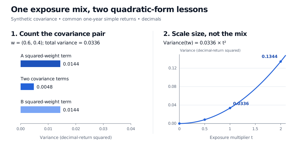
Original synthetic example. The left panel separates the three terms; the right keeps the exposure mix fixed and scales its size. Variance uses one-year decimal-return squared units.
Scale the position, then square the scale
Homogeneity means that for every real scalar ,
For the example, exposures have variance . Their standard deviation doubles to approximately 36.6606%. Reversing every exposure leaves variance unchanged because ; expected return and other economic consequences need not be unchanged.
The vector sums to 2. It describes leveraged risky-asset exposures relative to a capital base, rather than fully invested weights summing to 1. Borrowing, cash and financing costs must be specified separately. Deterministic financing changes the mean but adds no variance; uncertain financing can add variance and covariance terms. The scaling identity alone is not a complete financed-portfolio model.
Which forms can represent risk?
A general quadratic form can be positive, zero or negative. A covariance matrix must instead be positive semidefinite:
This is a condition on all directions, not on the signs of individual entries. The matrix with rows and has positive entries, yet its form at equals . It cannot be a covariance matrix. Conversely, negative off-diagonal covariances are perfectly compatible with nonnegative variance.
The example’s form can be written
Both coefficients are positive, and both squared terms vanish together only at the zero vector. This proves the example is positive definite. Positive semidefiniteness also permits nonzero zero-variance directions, such as those created by duplicate return series.
More generally, eigenvalue decomposition of symmetric , with orthogonal , transforms the form into , where . Nonnegative eigenvalues give a nonnegative form; mixed positive and negative eigenvalues give an indefinite form. This is the bridge from portfolio risk to curvature and quadratic programming. In optimisation, check whether the objective is written as or : their Hessians are and , respectively.
For the full sign classification and principal-axis geometry, continue with Quadratic Forms and Their Classification (public preview; full lesson requires membership).
Sources
- Gilbert Strang, Introduction to Linear Algebra, 5th edition, §6.5, “Positive Definite Matrices”: quadratic expressions, the doubled cross term, positivity tests and sums of squares.
- Andrew V. Sutherland, 18.782 Introduction to Arithmetic Geometry, Lecture 9, Fall 2013, Definition 9.1: homogeneous quadratic polynomials and their symmetric matrix representation.
- Penn State STAT 505, Linear Combinations of Random Variables, §2.3: variance as a covariance quadratic form.