Quadratic programming combines a quadratic objective with linear constraints. See how a return floor changes a minimum-variance portfolio, and when convexity guarantees a global solution.
Quadratic programming
Quadratic programming (QP) is optimisation of a quadratic objective function subject to linear equalities and inequalities. It is a natural language for portfolio construction: variance is quadratic in weights, while budgets, position caps and minimum expected returns can be linear.
“Programming” means selecting a plan. A QP describes the mathematical problem; a numerical algorithm is one way to solve it.
The objective is curved; the constraints are linear
A common minimisation form is
x∈Rnminsubject to21x⊤Qx+c⊤x,Ax=b,Gx≤h.
The vector x contains the decision variables. Take Q symmetric: the quadratic part is a quadratic form, while c⊤x adds a linear reward or cost. An additive constant changes the reported objective value but not the optimal point. Each row of the constraint matrices imposes one linear requirement; the intersection of those requirements is the feasible set.
The 1/2 is a convention that makes the gradient Qx+c. For portfolio variance w⊤Σw, the matching solver inputs are Q=2Σ and c=0. Choosing Q=Σ instead minimises half the variance. That gives the same weights when variance is the only objective term, but reports half the objective value. If a linear return reward is present, halving only the risk term changes the trade-off and can change the weights.
For example, minimising 2λw⊤Σw−μ⊤w uses Q=λΣ and c=−μ. The coefficient λ>0 specifies the risk penalty in that objective's units.
A return requirement moves the portfolio
Consider two hypothetical assets held for one year with fixed inception weights. Returns are simple total returns in a common currency. Stipulate these population moments:
Input
Asset A
Asset B
Expected return
8%
4%
Volatility
20%
10%
Return variance
0.04
0.01
Their covariance is zero. This is a model input, not a claim that the assets are independent. There is no cash asset, leverage, rebalancing or transaction cost. The weights must sum to one and remain nonnegative.
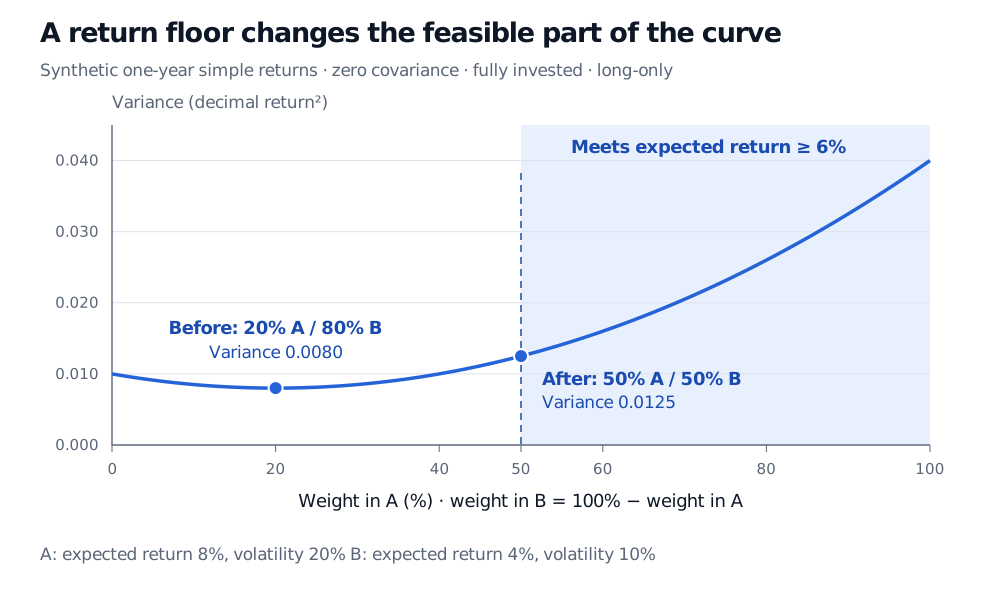
The completed square proves that the minimum is at wA=0.2, wB=0.8. Its variance is 0.008, volatility 0.008≈8.94%, and expected return 0.08(0.2)+0.04(0.8)=4.8%. The minimum occurs inside the budget segment, rather than at a corner as readers of linear programming might expect.
Now add a constraint: expected return must be at least 6%. Then
0.08w+0.04(1−w)≥0.06⟺w≥0.5.
The original optimum is no longer feasible. On the new interval [0.5,1], variance increases with w, since v′(w)=0.1w−0.02>0. The new optimum is therefore 50% A and 50% B, with
v(0.5)=0.04(0.5)2+0.01(0.5)2=0.0125.
Volatility rises to approximately 11.18% and expected return is exactly 6%. The return constraint binds here because lowering A's weight would reduce variance but violate the floor. An inequality need not bind in every QP: a 4% floor would leave the original 20/80 minimum feasible and optimal. Replacing “at least” with “exactly” would describe a different problem. A floor above 8% would be infeasible under these long-only rules.
Synthetic one-year variance curve with minimum at 20% A and variance 0.008, and return-constrained minimum at 50% A and variance 0.0125.
The objective curve stays fixed while the return floor removes allocations below 50% A. Shading marks the remaining feasible interval. Variance is in squared decimal-return units; all inputs are hypothetical.
Convexity provides the global guarantee
For symmetric Q, a positive semidefinite matrix makes the objective convex. Linear constraints give a convex feasible set. Together, these imply that every local minimum is a global minimum, if a minimum exists. An indefinite Q can produce a nonconvex QP; a local solver's answer then needs a separate global justification. Negative curvature confined to directions excluded by the constraints need not make the restricted problem nonconvex.
Convexity alone does not promise unique weights. Positive definiteness of Q is sufficient for uniqueness when a solution exists, because the objective is then strictly convex. A weaker sufficient condition is positive curvature along every nonzero direction joining feasible points. Thus a singular PSD matrix can still produce a unique constrained solution when the constraints remove its flat directions. Singular covariance is not, by itself, a reason to reject a portfolio QP or require a matrix inverse.
In the example, Q=2diag(0.04,0.01) is positive definite. Both feasible intervals are closed and bounded, so continuity ensures existence; strict convexity gives uniqueness.
What the answer does and does not establish
A quadratic risk constraint, such as w⊤Σw≤s2, is not a linear constraint. Combined with a quadratic objective, it gives a quadratically constrained quadratic programme rather than the ordinary QP above. Requiring integer share counts also changes the problem class. These distinctions determine which solver and optimality guarantees apply.
For a numerical result, inspect the achieved objective, budget residual, bound violations and optimality residuals under stated tolerances. Keep infeasibility separate from numerical failure. Then inspect the model: an exact optimum for estimated returns and covariances remains conditional on those inputs. Mean–variance optimisation does not establish that the expected return will be realised, or that variance captures every economically relevant risk.
For the derivation behind these guarantees, Constrained and Convex Optimisation develops multipliers, KKT conditions and convexity. The full lesson requires membership; a public preview is available.
Sources
Gérard Cornuéjols, Javier Peña and Reha Tütüncü, Optimization Methods in Finance, 2nd edition (2018), §5.1, pp. 71–73, and §6.2, pp. 93–94: QP structure and mean–variance portfolio formulations.