Choose the best feasible allocation, distinguish a boundary optimum from an unconstrained stationary point, and verify a squared-distance example with substitution and KKT conditions.
Constrained optimisation
Constrained optimisation chooses the best permitted values of a set of decision variables. An objective function ranks the choices, while constraints specify which choices are allowed. A portfolio can have an attractive model return and still be inadmissible because it exceeds its capital, position or exposure limits.
For a minimisation problem, a common formulation is
The inequalities can represent limits such as a maximum position size; the equalities can represent exact requirements such as full investment. Variable bounds belong to the constraints too. The feasible set contains the points satisfying all of them. The task is to find a feasible point with the lowest objective value, rather than to minimise first and hope the answer satisfies the rules.
Projecting an allocation target onto a budget
Suppose a synthetic allocation model produces provisional target exposures of 2 capital units to strategy A and 1 to strategy B. Only 1 capital unit is available, all of it must be allocated, and neither strategy may be shorted. Write the chosen allocations as x and y. The raw target (2,1) requests three times the available capital.
Choose the feasible allocation closest to that target in ordinary Euclidean distance. Squaring the distance preserves its ranking and gives
x,yminf(x,y)=(x−2)2+(y−1)2,x+y=1,x≥0,y≥0.
The allocations are measured in capital units; the objective is measured in squared capital units. This is a stipulated target-deviation penalty, not portfolio variance, expected loss or a forecast of realised risk. It assigns equal importance to one unit of deviation in either strategy. A covariance-weighted risk objective would be a different model.
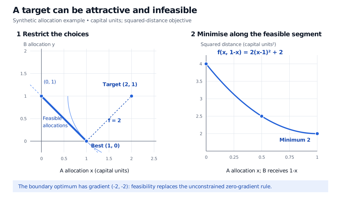
Without the constraints, the unique minimum is (2,1) with value zero. It is unavailable. With the constraints, substitute y=1−x. Nonnegativity restricts x to [0,1], so
f(x,1−x)=(x−2)2+x2=2x2−4x+4=2(x−1)2+2.
The square cannot be negative and vanishes only at x=1. Hence the unique global optimum is
(x∗,y∗)=(1,0),f(x∗,y∗)=2.
All capital goes to A under this particular objective. That result expresses the specified distance criterion and constraints; it does not establish that A is the better investment.
Synthetic allocation-target problem. Target (2,1) violates the one-capital-unit budget. The feasible segment joins (0,1) and (1,0); its closest point to the target is (1,0), with squared distance 2. Along the segment the objective is 2(x-1) squared plus 2, falling from 4 at x=0 to its unique minimum 2 at x=1.
Original synthetic target-distance example. The thick segment is the complete feasible set. The light-blue arc has objective value 2, and the right panel evaluates the objective only on feasible allocations.
Simply normalising the raw target to sum to one gives (2/3,1/3). That allocation is feasible, but its objective is 20/9>2. Normalisation and closest-point optimisation implement different rules. Neither procedure can be selected without deciding what the allocation is meant to optimise.
Why a nonzero gradient can be optimal
For differentiable unconstrained optimisation on an open domain, a local minimum must have zero gradient. At the constrained solution above,
∇f(1,0)=(−2,−2)=(0,0).
Increasing both allocations would reduce the objective initially, but it would break the budget. Along the budget, every feasible move away from (1,0) has the form (1−t,t) for 0<t≤1, and its objective increases by exactly 2t2. There is no feasible improvement.
Lagrange multipliers account for equality constraints. The Karush–Kuhn–Tucker conditions, or KKT conditions, also account for inequalities. Using inequalities −x≤0 and −y≤0, form
L=f+λ(x+y−1)−μxx−μyy,μx,μy≥0.
At (1,0), choose λ=2 and μx=μy=0. Then the gradient of the Lagrangian vanishes, all constraints hold, and complementary slackness holds: μxx=μyy=0.
The lower bound y≥0 is an active constraint because it holds with equality, yet its multiplier is zero. Active does not automatically mean a strictly positive multiplier. Here the budget-only closest point already has y=0; removing nonnegativity leaves the minimum unchanged.
These conditions need assumptions. For continuously differentiable objectives and constraints, linear independence of the equality gradients and active inequality gradients at a local minimum is one sufficient constraint qualification for KKT necessity. It holds here: (1,1) and (0,−1) are independent. For a convex differentiable objective, convex differentiable inequality functions and affine equalities, a feasible KKT point is globally optimal. Outside that convex setting, satisfying KKT alone does not prove a global minimum.
What the constraints change in a financial model
This example is a quadratic programme: the objective is quadratic and all constraints are linear. Its objective is strictly convex and its feasible set is convex, giving at most one minimiser; continuity on the nonempty closed, bounded segment also ensures existence. General constrained problems can instead be infeasible, unbounded, nonconvex or have several equally good solutions.
In mean–variance optimisation, the objective can be portfolio variance, with a full-investment equality, a minimum-return inequality and position bounds. Calibration can impose parameter positivity. Execution can impose a maximum participation rate. In each case, the constraints are part of the model of what can be done.
For minimisation, adding restrictions while keeping the same objective and its units can only leave the best attainable value unchanged or make it higher, provided the compared minima exist. It may also remove every feasible point. A higher constrained minimum is therefore not necessarily a solver failure. Conversely, a low reported objective is unhelpful if the returned allocation violates a budget or position limit. Numerical work should report feasibility residuals and tolerances alongside the objective.
For the equality method, inequality conditions and a genuine minimum-variance portfolio derivation, continue with Constrained and Convex Optimisation. The public page is a preview; the complete lesson requires membership.
Sources
Gérard Cornuéjols, Javier Peña and Reha Tütüncü, Optimization Methods in Finance, 2nd edition (Cambridge University Press, 2018), §5.1 (quadratic programmes and asset allocation), §5.4 (duality and optimality conditions), and Appendix A.2 (convex sets and functions).