Optimise an objective without added constraints: solve a two-variable loss, distinguish stationarity from optimality, and see what changes at a boundary.
Unconstrained optimisation
Unconstrained optimisation means choosing decision variables to minimise or maximise an objective without additional equality or inequality constraints. A common form is
x∈Rnminf(x).
The decision variables are what you choose; the objective function measures how good each choice is. In quantitative work, that objective might be a pricing-error loss or a model's negative utility. Calling the problem unconstrained describes the permitted choices, not how easy the objective is to optimise.
The function's domain still matters. An objective containing logx is defined only for x>0, even if no separate “subject to” line appears. In the usual smooth unconstrained setting, the domain is open and derivative tests apply at interior points. Removing written constraints does not make undefined parameter values usable.
A loss surface with a clear answer
Suppose a researcher chooses two signed factor tilts, x and y, measured in standardised, dimensionless units. A synthetic loss penalises deviation from the target (2,−1):
f(x,y)=(x−2)2+2(y+1)2,(x,y)∈R2.
The coefficient 2 makes a unit deviation in y twice as costly as the same deviation in x. Both positive and negative tilts are allowed. This is a weighted target-distance penalty: it is not a financial variance estimate, and it contains no budget, leverage, execution-cost or risk model.
The gradient collects the first derivatives:
∇f(x,y)=(2(x−2)4(y+1)).
Setting both components to zero gives x=2 and y=−1. This is the only stationary point. We can establish much more than stationarity: both squared terms are nonnegative, so
f(x,y)≥0=f(2,−1),
with equality only at (2,−1). Thus (2,−1) is the unique global minimiser, and 0 is the minimum value. The chosen point and the achieved objective value are different objects.
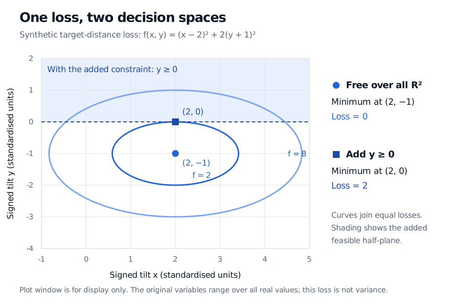
Synthetic dimensionless loss contours at values 2 and 8, centred on the unconstrained minimum (2, minus 1), where loss is zero. Adding y at least zero restricts choices to the shaded upper half-plane and moves the minimum to (2, 0), where loss is 2.
Original synthetic target-distance example. Curves join equal losses; the shaded half-plane applies only after adding the constraint. The displayed axis limits do not restrict the original problem.
Now add y≥0. The unconstrained solution is unavailable. For permitted values of y, (y+1)2≥1, with equality at y=0; independently, (x−2)2 is smallest at x=2. The new answer is (2,0), with loss 2. Its gradient is (0,4)⊤, which is not zero. Reducing y would lower the loss, but that direction is forbidden at the boundary. This is now constrained optimisation, requiring conditions that respect feasible directions.
What derivatives certify
For a differentiable objective, an interior local minimum must have zero gradient. That necessary condition is not a sufficient one. For example, g(u,v)=u2−v2 has zero gradient at (0,0), yet increasing u raises the objective and increasing v lowers it. The origin is a saddle point.
For a twice continuously differentiable function near a stationary point, the Hessian matrix supplies a local test:
Hessian at the stationary point
Conclusion
Positive definite
Strict local minimum
Negative definite
Strict local maximum
Indefinite
Saddle point
Semidefinite but not definite
The test alone is inconclusive
In the target-distance example,
H=(2004),h⊤Hh=2h12+4h22>0for h=0.
The Hessian is positive definite, confirming a strict local minimum. A positive-definite Hessian at one point is a local certificate; it does not exclude a lower minimum elsewhere. Here it is positive definite everywhere, making the quadratic strictly convex. The completed-squares argument already proved the global result directly. More generally, for a differentiable convex function on an open convex domain, a zero gradient certifies a global minimum; strict convexity makes any minimiser unique. These distinctions are developed in Boyd and Vandenberghe's Stanford slides, Chapter 9.
A solver still needs a model and a stopping rule
When the stationary equations cannot be solved explicitly, methods such as gradient descent generate successive candidate points. A small gradient is useful numerical evidence of approximate stationarity. Without further structure, it does not prove global optimality, and a numerical method can be sensitive to its starting point and step size.
Existence also needs attention. The unconstrained objective f(t)=e−t is positive for every real t and approaches zero as t→∞. Its infimum is zero, but no finite decision attains it. “Unconstrained” does not promise a solution.
For financial calibration, decide first which parameters must remain positive or bounded and how the loss scales different errors. A change of variables can absorb a restriction—for example σ=ez ensures positive volatility—but zero volatility then requires a limit rather than a finite z. The transformed problem's derivatives and numerical behaviour also change.
The Unconstrained Optimisation lesson extends this toolkit to quadratic utility, squared pricing error and Newton steps. Its public page is a preview; the full lesson requires membership.
Sources
Steven G. Krantz and Harold R. Parks, Vector Calculus (CRC Press, 2024), §3.8.1, “The Analogue of Fermat's Theorem,” and §3.8.3, “The Second Derivative Test for Local Extrema.”