Odds compare the probability that an event occurs with the probability that it does not. If an event has probability , its odds in favour are
Probability divides the event's weight by the whole. Odds divide it by the weight of the complementary event. The event, horizon and information set must stay the same in both quantities: default within one year is a different event from default within five years.
One default for every four nondefaults
Suppose a hypothetical credit model assigns a borrower a 20% probability of default within one year. This is a stipulated teaching probability, not an estimate for any real borrower. Its odds in favour of default are
Read this as one default per four nondefaults in the model's expected composition. In a synthetic population of 100 equivalent cases, that means 20 expected defaults and 80 expected nondefaults. It does not promise exactly those realised counts.
The odds against default reverse the ratio: , or . Always say in favour or against when a ratio might be ambiguous. An odds value of 0.25 is not a 25% default probability: the denominator is 80 rather than 100.
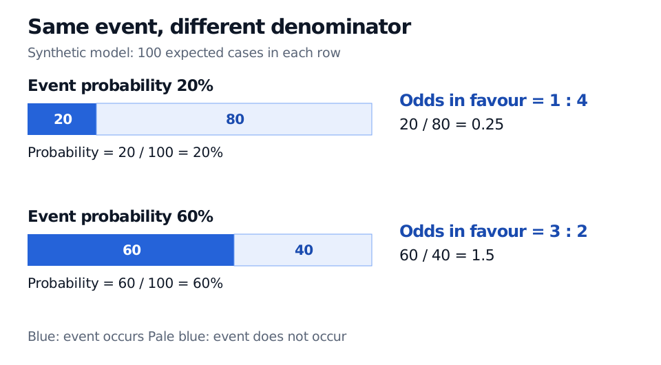
Original synthetic expected-count illustration. Probability compares the blue part with the whole bar; odds compare blue with pale blue.
Converting back, and what happens at the ends
Solving for gives
For finite nonnegative odds , probability is . Equivalently, odds mean three event cases out of five total cases. Odds greater than one are perfectly valid; probabilities greater than one are not.
| Probability | Odds in favour | Meaning |
|---|---|---|
| Zero probability under the model | ||
| Event is less likely than its complement | ||
| Event and complement have equal probability | ||
| Event is more likely than its complement | ||
| Approaches | Grows without bound | Complement becomes vanishingly unlikely |
At , the finite quotient divides by zero. It is conventional to write infinite odds using the extended nonnegative numbers, consistent with the limit as approaches one. For , odds against are the reciprocal of odds in favour. Endpoint statements need the corresponding zero/infinity convention. MIT's Bayesian Updating: Odds develops these conversions.
Why an alert multiplies odds
The odds form of Bayes' theorem separates the starting belief from the information in an observation. For a hypothesis and observed event , with positive conditioning probabilities and finite ratios,
The last factor is the likelihood ratio for this observation: posterior odds = prior odds × likelihood ratio.
Keep the 20% default prior. In an original toy alert model, suppose the alert occurs for 80% of defaults and 20% of nondefaults. Its likelihood ratio is . Prior odds become posterior odds , hence a 50% posterior default probability. A separate count check gives 16 alerted defaults and 16 alerted nondefaults among the 100 expected cases: .
Multiplying probability directly by four would give 80%, which is wrong. Nor is an alert's 80% detection rate the posterior probability of default. Both mistakes discard the starting composition. These results depend on the assumed prior and alert rates; odds algebra cannot establish whether those inputs describe a real credit population. If the evidence has zero probability, conditioning is undefined rather than an invitation to multiply zero by infinity.
Log-odds also appear in classification: for , ranges over the real line. In logistic regression, a linear predictor describes log-odds, with probabilities recovered through the inverse transformation. For that next step, the membership lesson Exponential Families, especially Example 1, derives the Bernoulli log-odds parameter; its public page provides a preview.
Statistical odds and quoted payouts
The definition here describes event probabilities. A betting quote may instead describe net winnings per unit stake or a total-return multiplier including the stake. Those conventions use different numbers. An implied probability inferred from a payout additionally needs a pricing assumption; a commercial quote can contain margins and need not equal a measured physical chance. State the convention before converting a quote.
An odds ratio is different again: it compares the odds of an event across two groups. A single event's odds are only one input to that comparison.
Sources
- Sheldon Ross, A First Course in Probability, 10th edition, Chapter 3, discussion of odds and equation (3.3): odds-form Bayesian updating.
- Jeremy Orloff and Jonathan Bloom, MIT 18.05, Spring 2022, Class 12: Bayesian Updating: Odds, §§2–4: conversion formulas, complementary odds and updating.