Probability assigns an event a number between 0 and 1 that describes its likelihood under a specified model and information set. It is dimensionless: 0.02 and 2% express the same probability. A statement such as “2% chance of loss” needs an instrument or strategy, a definition of loss and a time horizon before it can guide a decision.
Probability measures how likely an event is, while its financial consequence requires a separate payoff or random variable. A small probability can accompany an enormous loss.
A coherent probability law
The sample space contains the model's possible outcomes. A probability law assigns probabilities to its measurable events. In a finite model, every subset can be an event. The defining rules are:
- Nonnegativity: .
- Total probability one: .
- Countable additivity: for pairwise disjoint events ,
For finitely many exhaustive outcomes, assign nonnegative weights summing to one; an event's probability is the sum of the weights it contains. The outcomes need not be equally likely. Counting favourable outcomes and dividing by the total works only when equal likelihood is justified.
The rules imply , probabilities cannot exceed 1, and a complementary event satisfies . Additivity applies directly to disjoint events; overlapping events need their intersection subtracted to avoid double counting.
A trade that wins 98% of the time—in the model
Consider one hypothetical trade over a fixed period. Its two exhaustive outcomes are a gain of USD 2,000 with probability 0.98 and a loss of USD 100,000 with probability 0.02. These are stipulated net P&L amounts, with no additional costs in the example.
| Outcome | Probability | P&L (USD) | Probability × P&L (USD) |
|---|---|---|---|
| Win | 0.98 | +2,000 | +1,960 |
| Loss | 0.02 | −100,000 | −2,000 |
| Total | 1.00 | — | −40 |
The loss event is the complement of winning here because no break-even outcome exists. In a richer model, “does not win” may include both loss and zero P&L.
The expected value of P&L combines probability with magnitude:
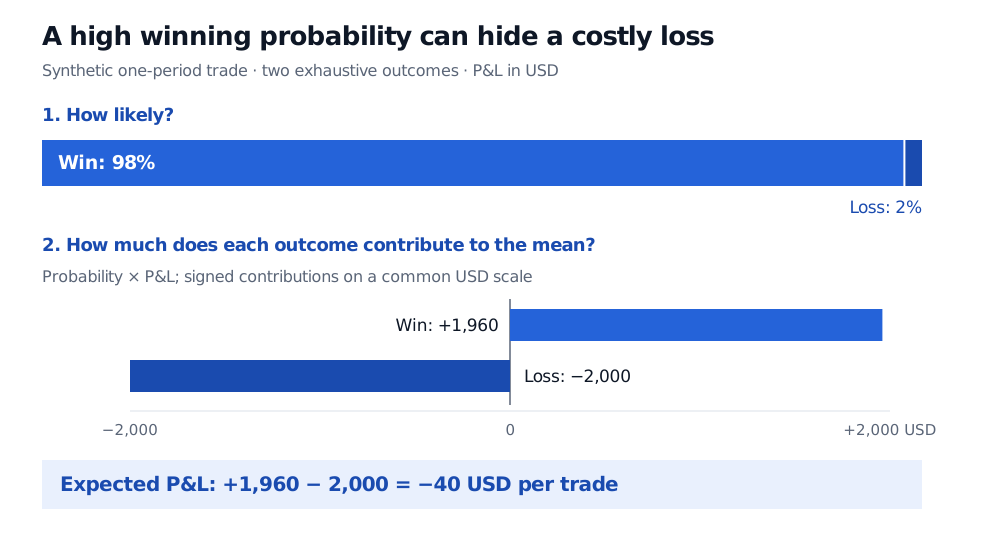
Original stipulated one-period model. The top bar shows probability mass; the lower bars show signed contributions to expected P&L in USD, using a different scale.
A 98% winning probability therefore coexists with negative expected P&L. The mean is also neither of the two possible realised outcomes. Neither winning probability nor expectation alone describes the capital needed to survive the large loss.
A model weight is not a promised frequency
The 0.98 above is an assumption, not evidence that a real strategy wins that often. An observed win fraction is an estimate tied to a population, sampling design, horizon and definition of profit. Its uncertainty matters; dependence between trades and changing market conditions complicate inference. The law of large numbers connects frequencies to probabilities under stated assumptions, not by guaranteeing exactly 98 wins in each 100 trades.
Likewise, zero probability is not a universal synonym for logical impossibility. In a continuous random variable model uniform on , any exact point, including , has probability zero even though it lies in the support: every sufficiently small neighbourhood around it has positive probability. The empty event is impossible, but an event with probability zero need not be empty. Omitting a crash state from a finite trading model also provides no evidence that an actual crash cannot occur.
For a fuller foundation, Probability Fundamentals develops event operations, conditioning and independence. Its public page is a preview; the full lesson is available with a free signed-in account.
Sources
- Dimitri P. Bertsekas and John N. Tsitsiklis, Introduction to Probability, 2nd edition, Athena Scientific, 2008, §1.2 (probabilistic models, axioms and models versus reality), §2.4 (expectation) and §3.1 (continuous random variables).
- MIT OpenCourseWare: selected textbook summary material, §§1.2 and 2.4, gives the probability axioms, finite laws and probability-weighted expectation.