Separate a statistic’s repeated-sample law from individual outcomes and one observed empirical distribution, using exact mean and variance calculations and contrasting sampling designs.
Sampling distribution
A sampling distribution is the probability distribution of a statistic when the sampling procedure is repeated under a specified population model or sampling design. It describes how a sample mean, sample variance or another calculated summary varies across possible datasets of the stated size.
For a quant estimating average trade P&L, this is the distribution that measures the estimate's sampling uncertainty. A histogram of individual trade outcomes answers a different question: how variable are the trades themselves?
Keep three distributions separate
Let T=T(X1,…,Xn) be a statistic computed from a sample. Before observing the data, T is random. After observing x1,…,xn, its realised value t=T(x1,…,xn) is a number.
Three objects then need distinct names:
Object
What is distributed?
What determines it?
Population distribution
An individual outcome X
The stipulated outcome model, or a declared weighting of the fixed finite population's values
Observed empirical distribution
The recorded values in one dataset
The realised observations, each assigned mass 1/n, with ties combined
Sampling distribution of T
The statistic across possible samples
The population, sampling design, sample size and chosen statistic
An empirical distribution can estimate the population law. It is not itself the sampling distribution of the mean. Likewise, a sampling distribution is not a posterior distribution expressing uncertainty about a parameter: in the usual frequentist setup, the parameter is fixed while the sample varies. Shao's lecture on statistics and their distributions develops this distinction between the random statistic and its observed value.
Four samples are enough to see the mechanism
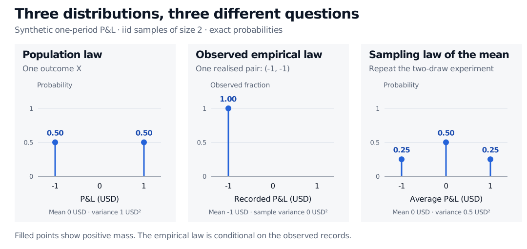
Use a synthetic fixed-position, one-period P&L model: each observation is USD -1 or USD 1, each with probability 1/2. The population mean is zero and its variance is 1USD2. Draw two observations independently from this law. This is an iid random sample, not sampling two distinct records without replacement.
The mean's standard error, the standard deviation of this sampling distribution, is 0.5≈0.7071 USD. Individual P&Ls still have standard deviation USD 1. Averaging reduces the uncertainty of the mean; it does not reduce the dispersion of the underlying trades. Berkeley's Standard Error explains this square-root relationship for independent draws.
Three exact distributions in a synthetic USD P&L model. Individual outcomes -1 and 1 each have probability 0.5. The observed pair (-1, -1) has empirical mass 1 at -1. Across iid pairs, the mean takes -1, 0 and 1 with probabilities 0.25, 0.50 and 0.25.
Original exact enumeration, not market data or simulation. The middle panel conditions on one realised pair; the right panel considers all four possible pairs.
If the observed pair happens to be (−1,−1), its empirical distribution places all its mass at USD -1. Its observed sample variance is zero. Neither observation changes the stipulated population law or proves that future trades have zero risk.
Changing the statistic changes the sampling distribution even with the same data-generating process. Here S2 takes values 0 and 2USD2, each with probability 1/2. Thus E[S2]=1USD2: it is unbiased under this model, although neither possible realised estimate equals the population variance.
Sampling design is part of the answer
Now change the experiment. Suppose there are exactly two fixed historical records, one at USD -1 and one at USD 1. Select both without replacement, randomising their order. The only ordered samples are (−1,1) and (1,−1), each with probability 1/2. Their mean is always zero: its sampling distribution is a point mass at zero, with zero variance.
Each individual draw has the same marginal distribution as before, but the draws are dependent. The change in sampling design changes the mean's law. A census removes sampling uncertainty about that finite pool, not uncertainty about future P&L. For larger pools, sampling without replacement requires the corresponding finite-population calculation.
For iid observations with mean μ and finite variance σ2,
E[Xˉ]=μ,Var(Xˉ)=nσ2.
Dependence can change this variance through covariance terms. More consecutive financial observations therefore do not automatically supply the information of the same number of independent observations.
Exact laws, approximations and inference
The two-point example needs no normal approximation. Its mean has three possible values; its sample variance has two. Neither law is normal.
With iid normal observations, the mean is exactly normal at every sample size. With iid observations having finite, positive variance, the central limit theorem instead gives a limiting result for the standardised mean:
σn(Xˉ−μ)dN(0,1).
This does not make every statistic normal, the raw observations normal, or every finite-sample tail approximation accurate. There is no universal sample-size cutoff. Infinite variance falls outside this version of the theorem; dependent observations need other conditions.
Sampling distributions underpin standard errors, confidence intervals and hypothesis tests. In real research the population law is usually unknown. Analytical assumptions, model simulation or a justified bootstrap supply an exact law or an approximation; they do not reveal it automatically from one dataset.
Populations, Samples, and Sampling Distributions develops the iid mean and normal-family calculations (public preview; full lesson requires membership). Simulation and Resampling shows how model simulation and bootstrap resampling address different uncertainty questions, including the limits of iid resampling for dependent returns (public preview; full lesson requires membership).
Sources
Casella, G. and Berger, R. L., Statistical Inference, 2nd ed., §5.2, especially Definition 5.2.1 and Theorem 5.2.6; §5.5, Theorem 5.5.15 for the finite-variance iid CLT.
Rice, J. A., Mathematical Statistics and Data Analysis, 3rd ed., §§7.2–7.3, especially §7.3.1: sampling distributions under simple random sampling from a finite population.