Sampling without replacement excludes repeat units. See how uniform finite-population sampling creates dependence and reduces the variance of an estimated ledger mean.
Sampling without replacement
Sampling without replacement means that a selected unit cannot be selected again in the same sample. An auditor checking a fixed ledger can choose each transaction at most once. Two different transactions may still have the same profit or loss: the restriction concerns record identity, not distinct numerical values.
The selection probabilities are a separate choice. Under simple random sampling without replacement, every subset of a specified size has the same probability. Choosing the first ten ledger rows also avoids repetition, but does not create a simple random sample. Measurement Canada's sampling definitions distinguish these two requirements explicitly.
This distinction matters when estimating a fixed book's average P&L. Equal-probability selection makes the ordinary sample mean unbiased, while the no-replacement rule reduces its sampling variance relative to independent uniform draws with replacement. Neither conclusion follows just from seeing a sample with no repeated records.
Three records, three possible pairs
Consider a synthetic ledger containing exactly three realised P&L records:
Record
Realised P&L, USD
A
−1
B
0
C
2
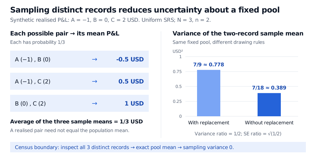
The target is this finite ledger's average, μ=(−1+0+2)/3=1/3 USD. Select two records by picking uniformly from all three, then uniformly from the two remaining records. Each ordered pair has probability (1/3)(1/2)=1/6. Each unordered pair has two orderings, giving probability 1/3:
Unbiasedness is a statement about averaging over the selection mechanism. None of these three possible sample means equals the population mean exactly.
Uniform sampling of two distinct records from synthetic P&L values of minus USD 1, USD 0 and USD 2 produces sample means minus USD 0.5, USD 0.5 and USD 1, each with probability one third. The sample-mean variance is 7/18 USD squared without replacement and 7/9 USD squared with replacement. Inspecting all three distinct records gives zero sampling variance.
Original synthetic fixed-ledger example. Uniform SRS without replacement halves the variance of the two-record mean; the standard error falls by the square root of one half. A census eliminates sampling error about this ledger.
The draws have the same marginals, but are dependent
Before observing either draw, each position is equally likely to contain A, B or C. Thus X1 and X2 have the same marginal distribution. Their conditional distributions change after a record is removed: if X1=−1, the second draw is equally likely to be 0 or 2, so its conditional mean is 1 USD. If X1=2, that conditional mean is instead −0.5 USD.
These draws are not independent. For a fixed population of N>1 values, define the divisor-N population variance as
σ2=N1k=1∑N(xk−μ)2.
Under sequential uniform sampling without replacement, two distinct draw positions satisfy
Cov(Xi,Xj)=−N−1σ2,i=j.
One way to see the negative covariance is to imagine randomly ordering the entire population. The total of all N draws is fixed, so its variance is zero. Every draw has variance σ2, and symmetry gives the same off-diagonal covariance c. Therefore 0=Nσ2+N(N−1)c, giving the identity above. This is negative when the population values vary, and zero when they are all equal. It describes dependence induced by selecting records; it does not estimate an economic relationship between different trades.
Here σ2=14/9 USD2, so Cov(X1,X2)=−7/9 USD2. Keeping that covariance in the variance of the average recovers the enumeration:
Var(2X1+X2)=41(914+914+2[−97])=187 USD2.
Dropping the covariance would give 7/9 USD2, the answer for two independent uniform draws with replacement. That mechanism allows the same record to be drawn twice, although any particular realised sample might happen to contain no repetition.
Use the finite-population correction with the right variance convention
For a uniform simple random sample of size 1≤n≤N, the exact result is
Var(Xˉ)=nσ2N−1N−n.
The factor (N−n)/(N−1) corrects the variance relative to independent uniform sampling with replacement. The corresponding correction to the standard error is its square root. In this example, the variance factor is (3−2)/(3−1)=1/2.
Survey-sampling texts also use a finite-population variance with divisor N−1:
S2=N−11k=1∑N(xk−μ)2=N−1Nσ2.
With that convention the same result becomes
Var(Xˉ)=(1−Nn)nS2.
Here S2=7/3 USD2, giving (1−2/3)(7/3)/2=7/18 USD2 again. Do not combine the divisor-N variance with the 1−n/N factor: that mixes conventions. When S2 is unknown and n≥2, the usual sample variance s2=∑i=1n(Xi−Xˉ)2/(n−1) is unbiased for S2 under this sampling design, so (1−n/N)s2/n estimates the variance of the sample mean.
At n=1, the exact variance is σ2. At n=N, the sample is a census: the mean is known exactly and sampling variance is zero. If N=1, the only nonempty sample is already a census; handle it directly rather than dividing by N−1.
For a small sampling fraction in a large population, the correction is close to one and an independence approximation may be useful. When a substantial share of the pool is sampled, it can materially overstate sampling error to ignore the correction. These are design-based statements about a fixed, complete sampling frame. Missing transactions, incorrect P&L fields, unequal selection probabilities and a changing population need separate treatment. A census of yesterday's ledger does not remove uncertainty about tomorrow's trading results.
For sequential probability calculations, see Example 2 in Conditional Probability, Total Probability, and Bayes' Rule. It works through the changing denominators in draws without replacement; the full lesson requires membership, with a public preview. When the recorded attribute is binary, the number of selected marked records under uniform SRS follows the hypergeometric distribution.
Sources
John A. Rice, Mathematical Statistics and Data Analysis, 3rd edition, Chapter 7, §§7.2–7.3, particularly Lemma B and Theorem B in §7.3.1 — finite-population moments and sampling-mean variance. Author-hosted Chapter 7.