Select every size-n subset with equal probability, enumerate a five-record fee audit, and distinguish equal inclusion from SRS and its finite-population variance correction.
Simple random sampling
Simple random sampling selects a fixed number of units so that every possible sample of that size has the same chance of selection. For the finite-population, without-replacement version used here, a selected unit cannot appear twice in one sample. The defining condition applies to entire samples, not just to individual units.
Let the population contain N labelled units and let the sample contain n distinct units, with 1≤n≤N. For every size-n subset s,
P(S=s)=(nN)1.
Here S is the random set of selected labels. Labels matter: two trades with identical fees are still two separate sampling units. This all-subsets definition is also the one in Measurement Canada's random-sampling specification, §3.1.13.
A fee audit with only ten possible outcomes
Suppose an operations analyst wants the average fee on a closed batch of five trade records. The synthetic fees are A: USD 0, B: USD 1, C: USD 2, D: USD 3 and E: USD 4. Reviewing two records is cheaper than reviewing the whole batch. The complete values are shown here so that we can evaluate the sampling rule; an actual audit would uncover only the sampled values.
There are (25)=10 possible unordered pairs. Select each with probability 1/10 and use its sample mean to estimate the batch average. Drawing uniformly from the five labels, then uniformly from the four remaining labels, produces this rule: AB can arrive as A-then-B or B-then-A, each with probability (1/5)(1/4)=1/20.
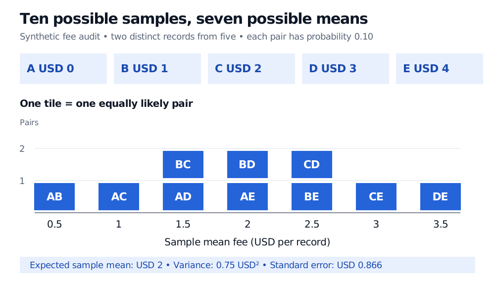
Ten equally likely two-record samples from synthetic fees A USD 0, B USD 1, C USD 2, D USD 3 and E USD 4. Their means range from USD 0.5 to USD 3.5. Counts at means 0.5, 1, 1.5, 2, 2.5, 3 and 3.5 are 1, 1, 2, 2, 2, 1 and 1. Expected mean is USD 2; variance is 0.75 USD squared.
Each filled tile represents one sample with probability 0.10. The distribution is exact enumeration of a synthetic fixed batch, not a simulation or a distribution of future fees.
The population mean is USD 2. Averaging the ten possible sample means gives
E[Yˉ]=100.5+1+1.5+2+1.5+2+2.5+2.5+3+3.5=2 USD.
The sample mean is an unbiased estimator: it is correct on average across repetitions of this selection procedure. A particular pair can still be misleading. AB gives USD 0.5 and DE gives USD 3.5; neither equals the true batch mean. Random selection gives a probability law for this error, not a guarantee that one sample looks representative.
Why equal chances for records are insufficient
Each record belongs to four of the ten possible pairs, so its inclusion probability is 4/10=2/5. In general, under this design,
πi=P(i∈S)=Nn,πij=P(i,j∈S)=N(N−1)n(n−1),i=j.
The pair formula applies when N>1. In the audit, πAB=1/10, whereas πAπB=(2/5)2=4/25. Inclusion events do not satisfy independence. Given that A is included, B's inclusion probability is 1/4, below its unconditional 2/5: A has used one of the two sample places.
Now change the procedure. Arrange the labels in the fixed cycle A–B–C–D–E–A and choose uniformly from its five neighbouring pairs: AB, BC, CD, DE and AE. Every record still occurs in two of five eligible pairs, so every inclusion probability is still 2/5. Yet AC, AD, BD, BE and CE can never be chosen. This is not simple random sampling.
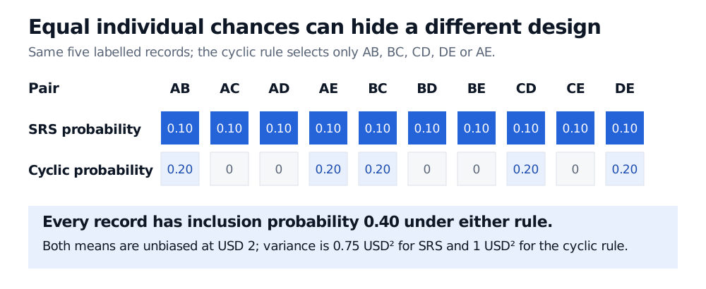
All ten pairs have probability 0.10 under simple random sampling. A cyclic alternative assigns probability 0.20 to AB, AE, BC, CD and DE, and zero to AC, AD, BD, BE and CE. Both designs include each record with probability 0.40 and have expected mean USD 2, but their sample-mean variances are 0.75 and 1 USD squared respectively.
Original design comparison for the same synthetic fees. Equal individual inclusion preserves the unbiased mean here, while the changed pair probabilities change its uncertainty.
The cyclic means are USD 0.5, 1.5, 2.5, 3.5 and 2. Their average is still USD 2, but their variance is 1 USD2, compared with 0.75 USD2 under SRS. Checking individual inclusion probabilities alone would miss that difference.
The finite-population correction, with the denominator visible
In design-based analysis, the values y1,…,yN are fixed. Randomness comes from which labels are selected. Define
μ=N1i=1∑Nyi,S2=N−11i=1∑N(yi−μ)2.
For N>1, simple random sampling without replacement gives
E[Yˉ]=μ,Var(Yˉ)=(1−Nn)nS2.
The factor 1−n/N is a finite-population correction for variance in this convention. Its square root enters the standard error. In the audit,
A second common convention uses σN2=N−1∑i(yi−μ)2, which is 2 USD2 here. The equivalent formula is
Var(Yˉ)=nσN2N−1N−n.
Do not combine the divisor-N variance with the factor 1−n/N; the correction and variance definition must match. With independent sampling with replacement, the variance would instead be σN2/n=1 USD2. Without replacement, later draws provide information about what remains, reducing uncertainty about this fixed batch mean. If n=N, the entire batch is observed and the design variance is zero.
When the population values are unknown and n≥2, estimate S2 using the observed sample variance s2=(n−1)−1∑i∈S(yi−Yˉ)2. Then
Var(Yˉ)=(1−Nn)ns2
is an unbiased estimator of the design variance. It varies with the selected sample. This does not make a normal or Student-t confidence interval exact for an arbitrary finite population; the audit's sampling distribution is the discrete distribution displayed above.
Make the sampling rule match the question
Start with a complete, deduplicated list of eligible records: the sampling frame. Assign each record a unique label and use a uniform without-replacement sampler, or a uniform random permutation followed by its first n labels. Record the frame, selection method and random seed so the selection can be reproduced. Decide the sample size before examining sampled fees; outcome-dependent stopping or substitutions change the design.
The target also matters. An unweighted sample average estimates the average per record. It does not automatically estimate a volume-weighted fee or an average per client. A random draw from a database that omits failed trades is only random within that database; it does not repair sampling bias in the frame. Missing fee records after selection need explicit handling rather than convenient replacements.
Finally, this calculation describes uncertainty about a fixed batch. Randomly selecting historical dates does not establish that future returns follow the same distribution, or eliminate market dependence. If guaranteed coverage of desks or trade types matters, stratified sampling can impose that coverage through a different design, whose variance must be analysed accordingly.
For a short introduction to population parameters, sample summaries and the independent-sample standard-error baseline, read Basic Statistics and Regression (public preview; full lesson free with a signed-in account).
Sources
John A. Rice, Mathematical Statistics and Data Analysis, 3rd edition, §7.2 and §7.3.1: finite populations, unbiased sample means and their variance under sampling without replacement.