Sampling bias systematically shifts an estimate away from its defined target. See why more selected returns can reduce noise without fixing coverage, and when reweighting helps.
Sampling bias
Sampling bias is systematic error caused by who can enter a dataset, who is selected, or whose outcomes are retained, relative to a defined target population and estimation procedure. A source can contain millions of accurately recorded returns and still overstate the mean return of the population you meant to study.
Bias is a property of the procedure across repetitions, rather than a label for every unbalanced sample. For an estimator μ^ of a target mean μ, its bias is
Bias(μ^)=E[μ^]−μ.
The expectation refers to the stated sampling and observation process. A particular sample can miss the population mean by chance even when this expectation equals the target. Conversely, one lucky estimate can equal the target even when the procedure is biased. Rice's survey-sampling chapter develops the distinction between an estimator being correct on average and fluctuating from sample to sample; the textbook reference is given below.
A return database with the wrong mix
Suppose a researcher wants the equally weighted mean one-period return across a specified universe of eligible security-return records. In a synthetic model, half the records concern liquid securities and half concern illiquid securities. Their group mean returns are +2% and −2%, respectively. Express returns in percentage points (pp), so the two numerical group means are +2 and −2.
The target mean is
μ=0.5(2)+0.5(−2)=0 pp.
The vendor's reported records instead have an 80% liquid / 20% illiquid mix. Assume reporting is representative within each group, so the reported group means remain +2 and −2 pp. Then an unweighted sample mean from independent draws from this reported-record distribution has expectation
E[Yˉn]=0.8(2)+0.2(−2)=1.2 pp.
Its bias for the target mean is +1.2 pp. The arithmetic is correct; the records answer a different population question.
One mechanism producing that mix is to report every liquid record but only one quarter of illiquid records. Starting with target masses 0.5 and 0.5, the retained masses are 0.5 and 0.125. Their total is 0.625, and conditioning on being reported produces shares 0.5/0.625=0.8 and 0.125/0.625=0.2. These are stipulated model probabilities, not estimates of any market or vendor.
If the intended target were reported records themselves, the same unweighted mean would be unbiased for that target's 1.2 pp mean. Calling a dataset biased without specifying its target and estimator leaves out the comparison that makes the claim meaningful.
Precision can improve around the wrong answer
To isolate the effect, now simplify the model so every liquid record returns +2 pp and every illiquid record returns −2 pp. Draw n reported records independently. The selected-record standard deviation is 1.6 pp, giving the exact standard error
SE(Yˉn)=n1.6 pp.
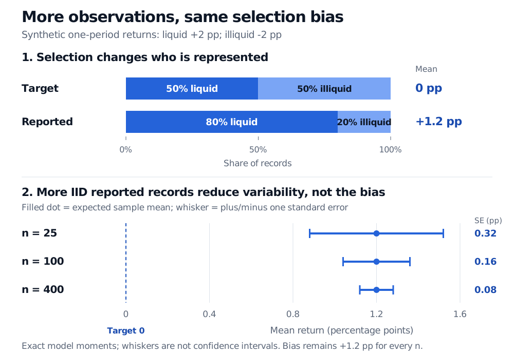
For 25, 100 and 400 records, this is 0.32, 0.16 and 0.08 pp. The expected mean remains 1.2 pp at all three sample sizes. Under these IID assumptions, the law of large numbers makes the mean converge to 1.2 pp as the sample grows. More data from the same selected distribution concentrate the estimate around that distribution's mean.
Synthetic return model: target records are 50% liquid and 50% illiquid with mean zero, while reported records are 80% liquid and 20% illiquid with mean 1.2 percentage points. For fixed within-group returns of +2 and -2 percentage points, standard errors are 0.32, 0.16 and 0.08 at sample sizes 25, 100 and 400; bias stays +1.2 percentage points.
Original synthetic model. In the lower panel, within-group returns are fixed at +2 and −2 pp. Whiskers show one standard error on either side of the expected sample mean; they are not confidence intervals.
This is the distinction between sampling variability and systematic selection. For the repeated-sample mean, random error is its movement around 1.2 pp; selection bias is the displacement of that centre from the target zero. Dependence between actual financial records changes the standard-error calculation and effective information. It does not, by itself, restore the missing population composition.
Selection can happen before a random number generator is ever used:
Undercoverage: a sampling frame covers one venue or only frequently traded securities, while the target includes others. Random selection within that frame does not give excluded records a chance to appear.
Nonresponse or selective reporting: returns may be absent more often for some managers, instruments or outcomes. Missing observations create bias when the observation process and estimator systematically distort the target quantity; missingness alone does not establish its direction or magnitude.
Survival filters: a historical study keeps only funds or securities that still exist today. Survivorship bias conditions the historical universe on later survival. Its effect depends on the target, outcomes and selection mechanism.
Sampling bias is part of the broader selection bias problem. It differs from measurement error: an included return may be recorded correctly even though the inclusion process is unsuitable. It also differs from future regime change. A representative historical sample need not describe tomorrow's market; that is an additional forecasting problem.
For a financial application, Corporate Actions and Survivorship explains historical eligibility, disappearing securities and terminal outcomes. The public page is a preview; the full lesson requires membership.
What would repair the example?
If the target group shares really are known to be 50/50, and the reported data identify each group's target mean, combine estimated group means using those target shares:
μ^group=0.5Yˉliquid+0.5Yˉilliquid.
Substituting the model group means recovers zero. Unequal selection is not inherently invalid: a deliberate stratified sample can use unequal inclusion rates and appropriate estimation weights. The failure here is applying the reported mixture's unweighted mean to a different target.
Reweighting has conditions. Both target groups must have positive coverage, the target shares must be defensible, and the observed group means must represent the corresponding target groups. If poor returns are less likely to be reported even within each liquidity group, balancing liquidity shares alone need not remove the bias. That requires further selection assumptions or sensitivity analysis. If an entire group has zero inclusion probability, ordinary inverse-probability weighting cannot recover its unobserved outcomes.
In practice, define the unit, eligibility dates, horizon and weighting target first; compare the frame and observed coverage against that target; then investigate which records disappear and why. A large sample size or a small standard error supplies no evidence that those coverage assumptions are correct.
Sources
John A. Rice, Mathematical Statistics and Data Analysis, 3rd edition, Duxbury, 2007, §§7.1–7.3: probability sampling, population parameters, unbiasedness and sampling variability. Numerical examples and figure here are original.