Sample every group, retain population weights, and quantify the trade-off between overall precision and subgroup coverage in a finite issuer universe.
Stratified sampling
Stratified sampling divides a population into non-overlapping groups, called strata, and selects a probability sample within every stratum. The groups together cover the target population. The analyst controls how much information comes from each group, then combines the results using weights that match the target quantity.
This is useful when a small but important group might barely appear in a simple random sample. A credit researcher can deliberately inspect more high-yield issuers, for example, while still estimating a mean across the whole issuer universe. Equal numbers inspected do not make the two groups equally important in that universe.
Ten from each group changes the mix
An analyst must manually reconcile one-month total returns for a fixed universe of 100 issuers. Before selecting any records, she splits it into two rating groups. This is a synthetic example; the true means below are supplied to check the sampling method and would normally be unknown.
Stratum
Issuers in universe
True mean return (pp)
Records sampled
A: investment grade
80
+2
10
B: high yield
20
−2
10
Here pp means percentage points: a return of 2 in the table is 2%, or 0.02 in decimal form. The target is the equal-issuer mean for this fixed month, not a capital-weighted portfolio return or an expected future return. Its true value is
μ=10080(2)+10020(−2)=1.2 pp.
Select ten issuers by simple random sampling without replacement within each group, independently across groups. Let yˉA and yˉB be the resulting stratum sample means. Pooling the twenty records with equal observation weights gives
yˉpool=21yˉA+21yˉB,Ed[yˉpool]=21(2)+21(−2)=0 pp.
The subscript d means expectation over repeated selections under the sampling design, holding all 100 returns fixed. The unweighted calculation targets a 50/50 mixture; the universe is 80/20. Its bias for the chosen target is therefore −1.2 pp. These are expectations, not claims that a particular sample has stratum means exactly +2 and −2.
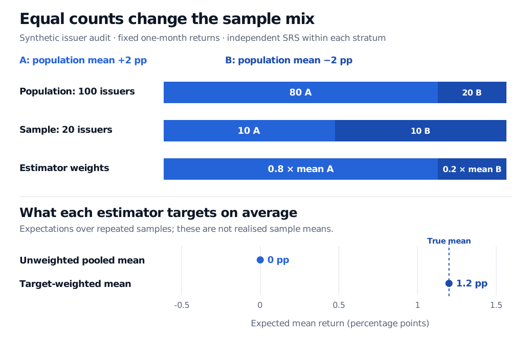
The synthetic population contains 80 A and 20 B issuers, but sampling ten from each makes a 50/50 sample. The estimator retains 80/20 population weights. Expected pooled mean return is 0 pp; expected target-weighted mean return is the true 1.2 pp.
Original synthetic fixed-month example. Bars distinguish population composition, sample allocation and estimation weights; markers show repeated-sampling expectations, not realised returns.
Restore the target with design weights
For stratum sizes Nh, total population size N, and stratum sample means yˉh, the stratified mean estimator is
μst=h=1∑HWhyˉh,Wh=NNh.
Each within-stratum simple-random-sample mean is unbiased for its own stratum mean. Linearity of expectation then makes this a design-unbiased estimator of the full population mean. Here it is 0.8yˉA+0.2yˉB, with expectation 1.2 pp. Unbiasedness does not mean every realised estimate equals 1.2.
The same correction can be expressed at the individual-record level:
Stratum
Inclusion probability per issuer
Inverse-probability design weight
A
10/80 = 0.125
8
B
10/20 = 0.5
2
Each selected A issuer represents eight population issuers; each selected B issuer represents two. Multiplying the observed returns by these weights, summing, and dividing by the known population count of 100 produces the same estimator. Do not confuse these expansion weights, 8 and 2, with the weights 0.8 and 0.2 applied to the two stratum means.
This argument assumes a complete sampling frame, correct group assignments and observed returns for all selected issuers. It does not repair missing failed issuers, selective data availability or a researcher replacing difficult records with convenient ones.
Precision follows the design
For independent simple random sampling without replacement within each stratum, with Nh>1 and 1≤nh≤Nh,
Here Uh contains all units in stratum h, μh is its true mean, and Sh2 is its finite-population variance, with divisor Nh−1. Independence refers to the selections across strata; issuer returns need not be independent draws from a market model for this design-based calculation.
For the example, additionally specify SA2=SB2=1 pp2. Then
Vard(μst)=0.82100.875+0.22100.5=0.058 pp2.
The standard error is 0.058≈0.2408 pp. This is a sampling-uncertainty scale, not a guaranteed error bound. The finite-population factors matter: ten records cover half of B. A census of a stratum makes its contribution zero. With unknown Sh2, use the within-stratum sample variances to estimate the design variance (at least two observations are needed in each non-census stratum); pooling all twenty records into an iid standard-error formula ignores this design.
Allocation is a choice about the question
Proportional allocation uses nh=nNh/N: with twenty observations here, that is 16 from A and 4 from B. Every issuer then has the same inclusion probability, so an unweighted pooled mean also has the correct population weights. Ten from each deliberately buys more information about B.
That trade-off is measurable. Under the specified equal stratum variances, proportional allocation gives overall-mean variance 0.040 pp², compared with 0.058 pp² for ten from each. But B's own sample-mean variance falls from 0.200 to 0.050 pp² when its sample grows from four to ten. The allocation that best estimates the full-universe mean need not be the allocation that best supports a subgroup report.
For a single overall mean, equal observation costs and known within-stratum standard deviations, Neyman allocation uses nh∝NhSh before integer, minimum-sample and census constraints. No design guarantees a variance improvement over simple random sampling for every stratification and allocation.
Finally, distinguish cluster sampling: stratification samples units from every group; cluster sampling selects groups themselves, then observes some or all units inside the selected groups. Also distinguish stratified sampling for simulation, where strata partition a model's probability space rather than a finite issuer list.
For a foundation in sample summaries, read Basic Statistics and Regression (full lesson free with a signed-in account; public preview available).
Sources
Rice, J. A. (2007). Mathematical Statistics and Data Analysis, 3rd ed., §§7.5.1–7.5.3: stratified random sampling, weighted estimation and allocation; §7.6: sampling-frame, response and measurement limitations.