Selection bias appears when the rule deciding which observations enter an analysis distorts the conclusion for the target population. An exact shortlist example shows how independent skill and luck signals can become negatively associated.
Selection bias
Selection bias is a systematic distortion of an inference caused by the mechanism deciding which observations enter or remain in an analysis. The key comparison is with the population and question the researcher meant to study. A perfectly calculated statistic can answer the wrong question if inclusion depends on information related to the outcome.
For a quant researcher, the first question is therefore “Which opportunities could have entered this dataset?” A file of voluntarily supplied analyst forecasts, completed orders or successful trading strategies may describe a selected subset. More observations from the same subset can estimate its properties very precisely while leaving the population inference distorted. Penn State's research-methods notes distinguish systematic selection error from random sampling error.
A shortlist can manufacture a relationship
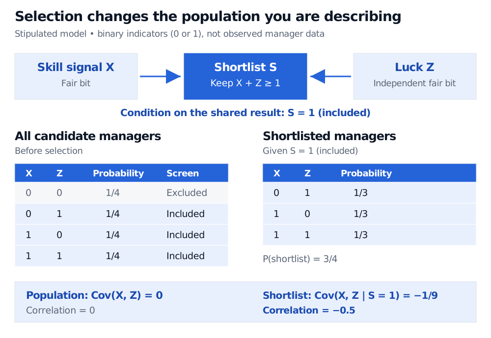
Consider an original, deliberately simplified manager-screening model. Let X be a binary skill signal and Z a binary indicator of favorable luck during evaluation. Stipulate that both are independent Bernoulli variables with probability 1/2 of equaling one. These are artificial model inputs, not measured manager skill or an empirical claim about how luck works.
The screen includes a manager if at least one input is favorable:
S=1{X+Z≥1}.
Every pair (X,Z) initially has probability 1/4. The screen removes only (0,0), so P(S=1)=3/4. Using conditional probability, each retained pair has probability (1/4)/(3/4)=1/3.
Skill signal X
Luck Z
Population probability
Probability given inclusion
0
0
1/4
0
0
1
1/4
1/3
1
0
1/4
1/3
1
1
1/4
1/3
Within the shortlist, a manager with X=0 must have Z=1. A manager with X=1 can have either luck outcome, with equal conditional probabilities. Thus learning that a shortlisted manager lacks the skill signal tells you they had favorable luck. In the full population, learning X told you nothing about Z.
A shared shortlist screen changes four equiprobable states into three equiprobable retained states. Full-population covariance is zero; shortlist covariance is minus 1/9 and correlation is minus 0.5.
Original stipulated binary model, not observed manager data. Both inputs determine inclusion; conditioning on their shared result changes the joint law.
The change can be calculated exactly. In the shortlist,
Each conditional variance is (2/3)(1/3)=2/9, giving correlation
Corr(X,Z∣S=1)=(2/9)(2/9)−1/9=−21.
Before selection, both covariance and correlation were zero. The negative association in the shortlist is a property of the screening rule; it does not establish a negative relationship between skill and luck in the candidate population, nor that increasing one causes the other to fall.
The mechanism diagram has two arrows pointing into inclusion: X→S←Z. Their shared result S is called a collider. Conditioning on a collider can create dependence between otherwise independent inputs. The sign is not universally negative: different inclusion rules can produce positive, negative or no association. The negative sign here follows from this particular “at least one favorable input” rule.
What changed: the law, the estimate, or the question?
Let Y be an integrable quantity of interest and S a zero-or-one inclusion indicator with P(S=1)>0. A useful identity is
E[Y∣S=1]−E[Y]=P(S=1)Cov(Y,S).
It follows by writing E[YS]=P(S=1)E[Y∣S=1]. Selection changes the mean when inclusion covaries with Y. Equal means alone do not establish that the whole distributions match or that other relationships are preserved.
This also clarifies three distinctions:
Sampling noise makes a finite estimate fluctuate around the law it samples. In the toy model the selected law itself has covariance −1/9, even before drawing a finite sample. Repeatedly collecting more shortlisted managers does not restore the population's zero covariance.
Survivorship bias is a particular selection problem: inclusion is conditioned on later survival or continued availability. Selective reporting can occur even when nobody disappears. Sampling bias commonly emphasizes how the sampling process misrepresents the target population; usage overlaps with selection bias.
A selected population can be the intended target. Describing skill–luck association among shortlisted managers is valid in this model. The error is treating that conditional association as the relationship among all candidates. A restrictive screen is not automatically a biased analysis.
Follow the inclusion rule back to the decision
Elton, Gruber, Brown and Goetzmann discuss a financial example in Modern Portfolio Theory and Investment Analysis: institutions control access to historical analyst forecasts and may be more willing to release records that evaluated well. The resulting archive can favor good historical performance even without superior underlying forecasting ability. The issue is access determined after performance is known.
A defensible research design specifies the target population, inclusion dates and eligibility rule before comparing performance. For analysts, obtain a prospectively defined forecast panel rather than relying only on favorable records released retrospectively. For backtests, retain failed trials and reconstruct the historical opportunity set. For execution studies, retain unfilled intentions when the question concerns the whole execution policy; restricting to fills changes the question.
Statistical correction requires assumptions about the selection mechanism. Heckman's sample-selection work develops model-based correction, rather than a universal adjustment applicable to every filtered dataset. Reweighting similarly needs justified inclusion probabilities and adequate coverage: if a relevant type has zero chance of observation, its outcomes cannot be recovered by assigning larger weights to the observed types alone. Seek additional data, narrow the target or state the unresolved sensitivity.
Larry Wasserman, All of Statistics: A Concise Course in Statistical Inference, §§17.3 and 17.5 — collider structure and conditioning in directed graphs.
Edwin J. Elton, Martin J. Gruber, Stephen J. Brown and William N. Goetzmann, Modern Portfolio Theory and Investment Analysis, 9th edition, Chapter 17, “Information in Analysts' Forecasts,” pp. 438–439 — selective access to historical forecasts.