See how imperfect measurements change regression targets: derive classical predictor-error attenuation, contrast noisy outcomes, and identify what a correction requires.
Measurement error
Measurement error is a difference between a recorded value and the quantity that the analysis intends to measure. A mistimed price, a misreported position or a noisy estimate of an exposure can change the apparent relationship between a trading signal and subsequent profit. The target must be defined first: a transaction price and a contemporaneous midpoint are different quantities, so their difference is an error only relative to a stated measurement objective.
Write an additive measurement model as
W=X+U,
where X is the target quantity, W its recorded measurement and U the measurement error. This notation does not establish that U is small, independent or mean zero. Those are additional assumptions. Errors can also involve rounding, incorrect categories, systematic scaling or nonlinear transformations rather than additive independent noise. Schennach's measurement-systems review distinguishes classical and nonclassical models.
Consider a synthetic population, not a historical backtest. A centred trading signal X takes values −1 and +1 signal units with equal probability. One-period profit is exactly Y=2X USD: the true slope is USD 2 per signal unit. A recording process adds noise U of −1 or +1 signal units, also equally likely and independent of X.
The four equally probable states are:
True signal X
Recording error U
Recorded signal W
Profit Y, USD
Probability
−1
−1
−2
−2
1/4
−1
+1
0
−2
1/4
+1
−1
0
+2
1/4
+1
+1
+2
+2
1/4
All variables have mean zero. Independent noise raises predictor variance without adding covariance with profit:
Var(W)=Var(X)+Var(U)=1+1=2,Cov(W,Y)=2.
The variances are in squared signal units; covariance is in USD times signal units. Consequently, the population slope of profit on the recorded signal, with an intercept, is
βW=Var(W)Cov(W,Y)=22=1 USD per signal unit.
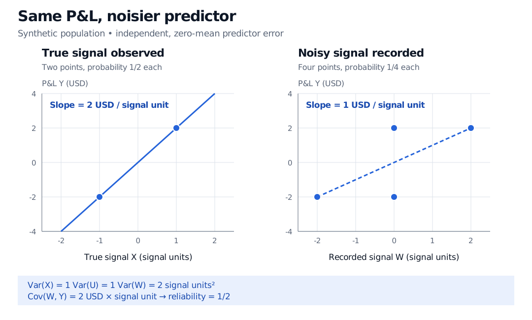
Synthetic population: the true signal X takes minus or plus 1 and profit Y is minus or plus USD 2. Independent recording noise produces four equally likely recorded-signal and profit pairs: (−2, −2), (0, −2), (0, 2), (2, 2). The population slope falls from USD 2 to USD 1 per signal unit.
Original synthetic population. The left panel shows the true relation; the right shows its population least-squares projection after independent predictor error. Filled markers are possible outcomes; lines are fitted relations, not time paths.
This is not an unlucky four-observation sample. The table specifies the whole probability law. Under independent repeated sampling from this law, the estimated slope converges to 1 as the sample grows. More observations sharpen the estimate of that slope; they do not recover 2.
The target matters. If the task is to forecast profit from the recorded signal available to the trader, slope 1 is appropriate here: E[Y∣W]=W, with the numerical value of W converted to USD. At a recorded zero, the two profits cancel in expectation. The problem arises when an analyst interprets this as the response to one unit of the unobserved true signal.
Assume finite second moments, positive Var(X), E[U]=0, Cov(X,ε)=0, and measurement error uncorrelated with both X and ε. Independence of U from the pair (X,ε) is a sufficient, stronger condition. With an intercept,
βW=βλ, reliability ratioVar(X)+Var(U)Var(X).
Thus 0<λ≤1. In the example, λ=1/2. Nonzero predictor-error variance pulls a nonzero population slope toward zero; a negative slope becomes less negative. Zero error variance gives λ=1, and a true zero slope remains zero under these assumptions. Under iid sampling, the sample OLS slope converges to this population value; the formula is not a claim that every finite-sample estimate, or its expectation, equals βλ.
Substitution reveals the source of endogeneity:
Y=α+βW+(ε−βU),Cov(W,ε−βU)=−βVar(U).
The observed predictor shares measurement noise with the composite disturbance. Changing standard errors does not remove this covariance. The Endogeneity and Instrumental Variables lesson develops the distinction between coefficient inconsistency and unreliable uncertainty estimates, then states the requirements for instruments. A public preview is available; the full lesson requires membership.
Attenuation is conditional on the model. If a calibration error instead records W=X/2 while Y=2X, the slope on W is 4, twice the slope on X. Correlated errors, multiple mismeasured predictors and nonlinear models do not inherit the simple scalar formula. A Berkson model reverses the construction: X=W+V with mean-zero V independent of W. In a linear model with Cov(W,ε)=0, regression on W retains slope β. Paciorek, Gryparis and Coull compare these two constructions.
A noisy outcome is a different problem
Now measure X correctly but observe Yobs=Y+V. If V has mean zero and is independent of (X,ε), the population slope on X stays β: the extra noise has zero covariance with the predictor. With finite noise variance, its variance adds to the disturbance variance, reducing precision for a fixed sampling design. For the synthetic Y=2X example, adding independent outcome noise of ±1 USD leaves slope 2 and introduces disturbance variance of 1 USD squared.
Outcome error can still bias slopes when it is related to predictors—for example, if larger positions systematically have more understated reported losses. “Measurement error causes attenuation” is therefore too broad, even before considering more complex models.
Nor is measurement error synonymous with model error or a residual. A true economic outcome may depart from a model's prediction even when recorded perfectly. A fitted residual combines whatever the regression has not explained; it does not identify the recording error. Indeed, OLS residuals are orthogonal to included predictors by construction, which cannot establish that those predictors were measured correctly.
What information would support a correction?
Start with the measurement process: timestamp alignment, currency and units, revisions, stale records and the definition of the economic quantity. Correct a confirmed data defect from its source where possible, preserving the original record and the reason for the change.
A statistical correction needs additional evidence. A validation sample with credible target measurements can estimate the error structure. Repeated readings can help if the target remains the same and their errors satisfy justified independence assumptions. Instrumental variables require relevance and validity for the composite disturbance; a correlated alternative feed is not automatically valid when both feeds share errors.
Within the classical scalar model, known reliability would permit dividing βW by λ. But the distribution of recorded W alone does not separate signal variance from error variance. Guessing λ merely supplies a new assumption, and estimating it adds uncertainty. When validation is unavailable, report sensitivity to plausible error structures rather than presenting a corrected coefficient as observed fact.
Sources
Jeffrey M. Wooldridge, Econometric Analysis of Cross Section and Panel Data, Chapter 4, §4.4.1, “Measurement Error in the Dependent Variable,” and §4.4.2, “Measurement Error in an Explanatory Variable,” especially equations 4.44–4.48.