Sampling with replacement keeps each record eligible for every draw. Enumerate repeated selections, compare mean variance, and understand bootstrap duplicates.
Sampling with replacement
Sampling with replacement selects a unit, records it, and returns it to the eligible pool before the next selection. The same unit can therefore appear more than once in a sample. In a historical-scenario calculation, that means a recorded trading day can be selected repeatedly; the algorithm does not consume the row when it uses it.
Replacement describes eligibility. Equal selection probabilities and independence are separate design choices. The common model makes each draw independently and uniformly from the same fixed pool. Under those assumptions, the draws are independent and identically distributed, even when the pool is small.
Three P&L records, nine possible samples
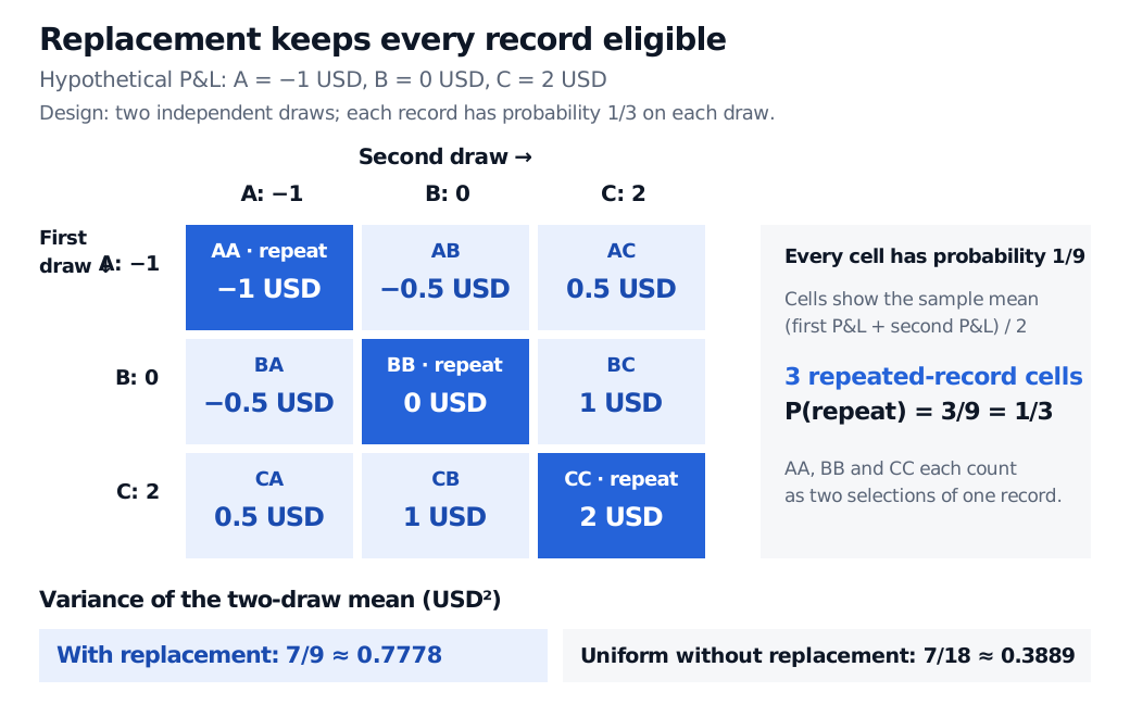
Suppose a researcher has three hypothetical, same-horizon P&L records, labelled A: −USD 1, B: USD 0, C: USD 2. Draw twice with replacement, independently, assigning each record probability 1/3 on each draw. These are stipulated sampling probabilities, not estimates of future market probabilities.
There are 32=9 ordered record pairs. For example, AB means first selecting A and then B, giving the sample mean (−1+0)/2=−0.5 USD. BA is a different ordered sample with the same mean. Each ordered pair has probability (1/3)(1/3)=1/9.
Nine equally likely ordered samples from hypothetical P&L records A of minus USD 1, B of USD 0 and C of USD 2. The three repeated-record pairs AA, BB and CC give repeat probability one third. Cells show sample means of minus 1, minus 0.5, 0, 0.5, 1 or 2 USD. The two-draw mean variance is 7/9 USD squared with replacement, versus 7/18 without replacement.
Two independent uniform draws from three fixed records. Each cell represents probability 1/9; blue diagonal cells repeat a record. All amounts are hypothetical USD P&L, and each cell displays the mean of its two selections.
The repeated-index event consists of AA, BB and CC, so
P(same record twice)=93=31.
Selecting the same record twice is allowed, not required. Also distinguish record identity from value: two different trading days can have identical P&L. Equal numerical values would not necessarily mean a repeated record.
Across the nine samples, the means −1,−0.5,0,0.5,1,2 have probabilities 1/9,2/9,1/9,2/9,2/9,1/9, respectively. This sampling distribution has expectation 1/3 USD and variance
Var(Xˉ)=2σ2=97 USD2≈0.7778 USD2.
No normal approximation is involved: enumerating all nine samples gives the result exactly.
What changes when replacement is removed?
Under independent uniform sampling with replacement from N fixed values, every ordered sequence of n record indices has probability N−n. The sample size can exceed N because repetition is permitted. If the pool mean and divisor-N variance are μ and σ2, then
E[Xˉ]=μ,Var(Xˉ)=nσ2.
There is no finite-population correction for these independent draws. By contrast, under uniform sampling without replacement, with N>1 and 1≤n≤N,
Var(Xˉ)=nσ2N−1N−n.
For our pool, the distinct two-record subsets AB, AC and BC have means −0.5,0.5,1 USD, each with probability 1/3. Their mean variance is 7/18 USD2≈0.3889 USD2, half the with-replacement value. This comparison uses the same divisor-N definition of population variance in both formulas. Sampling every record without replacement gives the finite census mean exactly; taking N draws with replacement need not visit every record.
That distinction matters for an audit of a fixed historical population. Selecting a previously seen record again is another random draw, but it does not reveal a new record from that census. If all three records are already known, their census mean is already calculable: resampling describes the variability of the chosen sampling mechanism rather than discovering the mean anew. Statistics Canada distinguishes the two designs through the possibility of repeat selection.
The drawing rule still matters
Uniformity cannot be inferred from replacement. An algorithm could independently select A, B and C with probabilities 1/2,1/3,1/6. Its repeated-index probability would be ∑ipi2=7/18, rather than 1/3, and its ordinary mean would target that weighted pool distribution.
Independence cannot be inferred either. Choose the first record uniformly, put it back, then deliberately choose the same record again. Both positions are marginally uniform, yet the second is completely determined by the first. Replacement is allowed throughout, while the repeat probability is one. The formula σ2/n relies on independence, which removes the covariance terms in the variance of an average.
Why the bootstrap allows duplicates
The ordinary nonparametric bootstrap draws independently with replacement from the empirical distribution, conditional on the observed data, and recalculates a statistic. A conventional bootstrap resample usually has the same number of rows as the original dataset: three here, rather than the two used above to make every pair visible. Wasserman's treatment separates approximating an unknown sampling distribution with the empirical distribution from the subsequent simulation step.
Resampling is useful for studying uncertainty, but the resampled rows are not new independent market observations. Ordinary row resampling does not preserve serial dependence in returns, recover unobserved crash scenarios, or establish that the historical pool represents the future. Bootstrap validity requires assumptions about the original data and the statistic; dependent time series may require a suitable block-based method. More resamples reduce simulation noise within the chosen bootstrap model, without fixing those assumptions.
For a seeded financial implementation and the distinction between simulation error and original-data uncertainty, see Simulation and Resampling (membership for the full lesson; public preview).
Sources
John A. Rice, Mathematical Statistics and Data Analysis, 3rd edition, §1.4.2 (ordered samples and replacement) and §7.3.1 (sample-mean variance and finite-population correction).