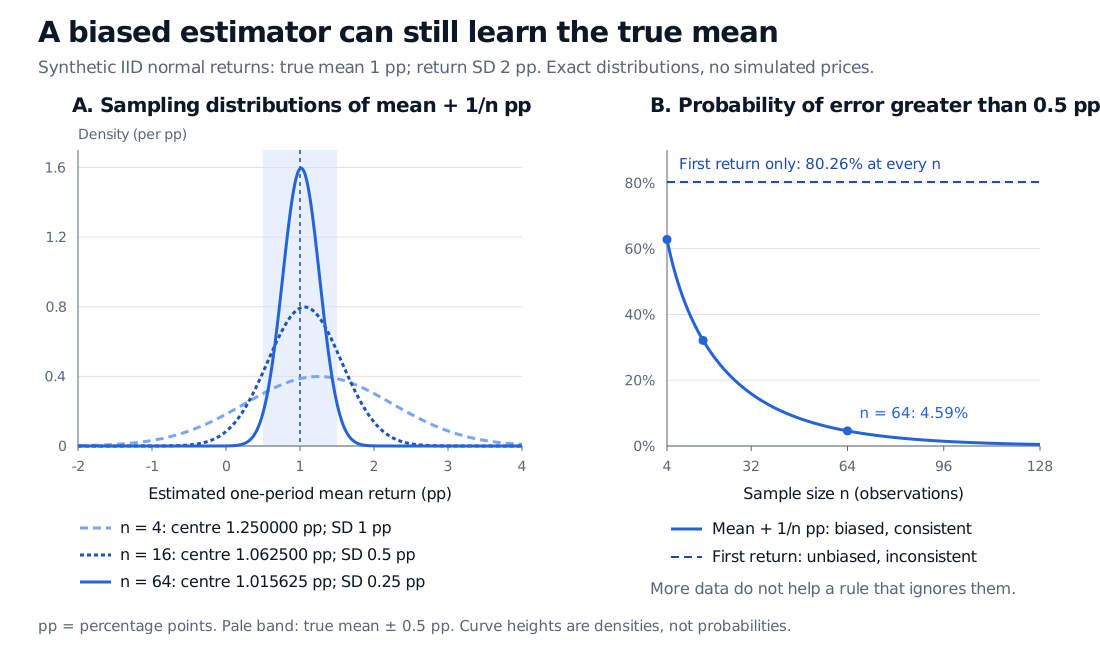
Consistency means a fixed-size estimation error becomes unlikely as the sample grows. Compare a biased but consistent return mean with an unbiased rule that never learns.
Consistent estimator
A consistent estimator is a sequence of rules for estimating a parameter whose probability of a fixed-size error tends to zero as the sample size grows. For a quant estimating expected return, consistency asks whether an ever-longer sample makes the estimate concentrate around the true mean, under the stated data model.
It is a large-sample property. It does not promise an accurate estimate from this year's data, and it does not require the estimator to be unbiased at every sample size.
What “concentrate” means
Let θ^n=Tn(X1,…,Xn) be an estimator of a fixed parameter θ. It is consistent for θ when
for every ε>0,n→∞limPθ(∣θ^n−θ∣>ε)=0.
This is convergence in probability, written θ^npθ. The probability is calculated under the data-generating model with true parameter θ. To call a procedure consistent throughout a model, this condition must hold for each parameter value in that model; the sample size needed can depend on θ.
Equivalently, choose any positive error tolerance ε and any positive failure-probability tolerance δ. Eventually, for every sufficiently large n, the probability of an error exceeding ε is below δ. You fix the tolerance first, then let the sample grow.
The statement concerns a sequence of sampling distributions. It does not say that every additional observation makes a particular realised estimate closer to the truth. A running return average can move away from its target before moving back.
A biased return estimate that still converges
Consider a synthetic model of independent, identically distributed one-period returns. Measure returns in percentage points (pp): a return of 1 in these units means 1%, not a decimal return of 1. Suppose
Xi∼N(μ,σ2),μ=1 pp,σ=2 pp.
The sample mean Xˉn=n−1∑i=1nXi is unbiased, with variance 4/n pp². Now deliberately add a small upward adjustment:
Tn=Xˉn+n1 pp.
This is a teaching device, not a proposed correction for trading data. Its bias is positive at every finite n:
E[Tn]−μ=n1 pp,Var(Tn)=n4 pp2.
The deterministic adjustment changes the centre, not the variance. Both its bias and its dispersion vanish as the sample grows.
Observations n
Mean of Tn (pp)
Bias (pp)
Standard deviation (pp)
Variance (pp²)
4
1.25
0.25
1
1
16
1.0625
0.0625
0.5
0.25
64
1.015625
0.015625
0.25
0.0625
These are properties across repeated samples, not three observed returns or a forecast path. Normality makes the plotted sampling distributions exact; a normal approximation is unnecessary here.
Exact synthetic IID normal example: mean plus 1/n pp has centres 1.25, 1.0625 and 1.015625 pp and standard deviations 1, 0.5 and 0.25 pp at n equal to 4, 16 and 64. Its probabilities of error greater than 0.5 pp are 62.79%, 32.11% and 4.59%. Using only the first return has an unchanged error probability of 80.26%.
Original exact-model comparison. True one-period mean 1 pp; return standard deviation 2 pp. The shaded band is the true mean ± 0.5 pp. Increasing sample size narrows the estimator's distribution, not the distribution of an individual return.
Markov's inequality applied to the nonnegative squared error gives, for any ε>0 measured in the same return units,
P(∣Tn−μ∣>ε)≤ε2E[(Tn−μ)2]⟶0.
The variance and squared bias shrinking to zero are a sufficient condition for consistency. They are not its definition: convergence in probability alone need not control expectations or second moments. The law of large numbers also gives a direct route: the sample mean converges, and the added adjustment vanishes. IID sampling with a finite first absolute moment suffices for the usual sample-mean law; the finite variance here makes the MSE proof especially short.
Unbiasedness cannot replace consistency
Suppose another analyst reports only the first return, regardless of how much data arrives:
Un=X1for every n.
This is an unbiased estimator of μ: E[Un]=μ. But its variance stays at 4 pp². More decisively, in this normal model,
P(∣Un−μ∣>0.5 pp)=2[1−Φ(0.25)]≈0.8026
for every n, where Φ is the standard normal cumulative distribution function. The error probability does not approach zero, so Un is inconsistent. Compare the two questions: unbiasedness concerns the sampling mean at a given sample size; consistency concerns concentration as sample size grows. Neither property guarantees the other.
What changes with actual return histories
The IID model above is an assumption, not a description of every market. With finite second moments and a common mean μ, the general variance calculation is
Var(Xˉn)=n21i=1∑nj=1∑nCov(Xi,Xj).
Autocorrelation introduces off-diagonal terms. If this variance tends to zero, the common-mean sample average is still consistent by the same probability bound. Dependence therefore requires a suitable argument; it does not automatically defeat consistency.
Conversely, stationarity alone is insufficient. If Xi=μ+Z for every observation, with the same nondegenerate normal shock Z of mean zero and variance 4 pp², the entire stationary history repeats one shock. Its average remains μ+Z, with variance 4 pp² at every sample size. Counting more rows has added no independent information.
A changing expected return raises another issue: what fixed parameter is the longer history supposed to estimate? A consistent estimate of a historical model's mean need not estimate the next regime's mean. A fixed-length rolling window also does not acquire this growing-sample guarantee merely because the calendar advances.
For the proof behind averaging and the distinction between concentration and normal error approximations, read Laws of Large Numbers and the Central Limit Theorem (public preview; full lesson requires membership).
Sources
George Casella and Roger L. Berger, Statistical Inference, 2nd ed., Duxbury, 2002, §10.1.1: Definition 10.1.1, Theorem 10.1.3 and Theorem 10.1.5. Definitions, vanishing-bias/variance criterion and vanishing deterministic adjustments.