Statistical power: Definition & Examples

Statistical power is the probability that a specified hypothesis test rejects its null hypothesis when a particular alternative is true. It measures a procedure's ability to detect an effect under a stated data-generating model. For a quant researcher, power answers a planning question: if an economically meaningful edge really existed, how often would this research design produce a rejection?

There is no meaningful standalone claim that “this test has 80% power.” Power must be attached to an effect, a sample size, a noise model, a rejection rule and a significance level.

Fix the rule, then change the truth

Let

R

be the rejection region and

\theta

the parameter governing the data. The power function is

\pi(\theta)=\mathbb{P}_{\theta}(X\in R).

At a specified alternative hypothesis

\theta_1

, this is

1-\beta(\theta_1)

, where

\beta(\theta_1)

is the Type II error probability: failing to reject when that alternative is true. The subscript matters. Missing a tiny effect and missing a large effect need not have the same probability.

The same function can be evaluated under the null hypothesis. There it gives a false-rejection probability. A test with significance level

\alpha

constrains that probability to be at most

\alpha

across the null. For the exact continuous test below, it equals

\alpha

at the point null. This is how one decision rule connects false alarms with successful detection; the rule stays fixed while the assumed truth changes.

A real edge can still produce an inconclusive history

Imagine a desk planning a fixed-length evaluation of one strategy, with returns measured in percentage points per observation. Use the deliberately simple model

X_1,\ldots,X_n\stackrel{\mathrm{iid}}{\sim}\mathcal{N}(\mu,\sigma^2), \qquad \sigma=2\text{ percentage points, known}.

These are stipulated normal returns, not market observations or a forecast. A value of $0.5$ in these units means a return of $0.5\%$ , not $50\%$ . No annualisation is applied. The desk predeclares $H_0:\mu=0$ against $H_1:\mu\ne0$ , at $\alpha=0.05$ .

For

n=100

, the sample mean's standard error is

\sigma/\sqrt n=0.2

percentage points. Under the null,

Z=\frac{\bar X}{\sigma/\sqrt n}\sim\mathcal{N}(0,1).

Writing $c=\Phi^{-1}(0.975)=1.95996398\ldots$ , the fixed rule rejects when $|Z|>c$ , or equivalently when

|\bar X|>0.3919928\text{ percentage points}.

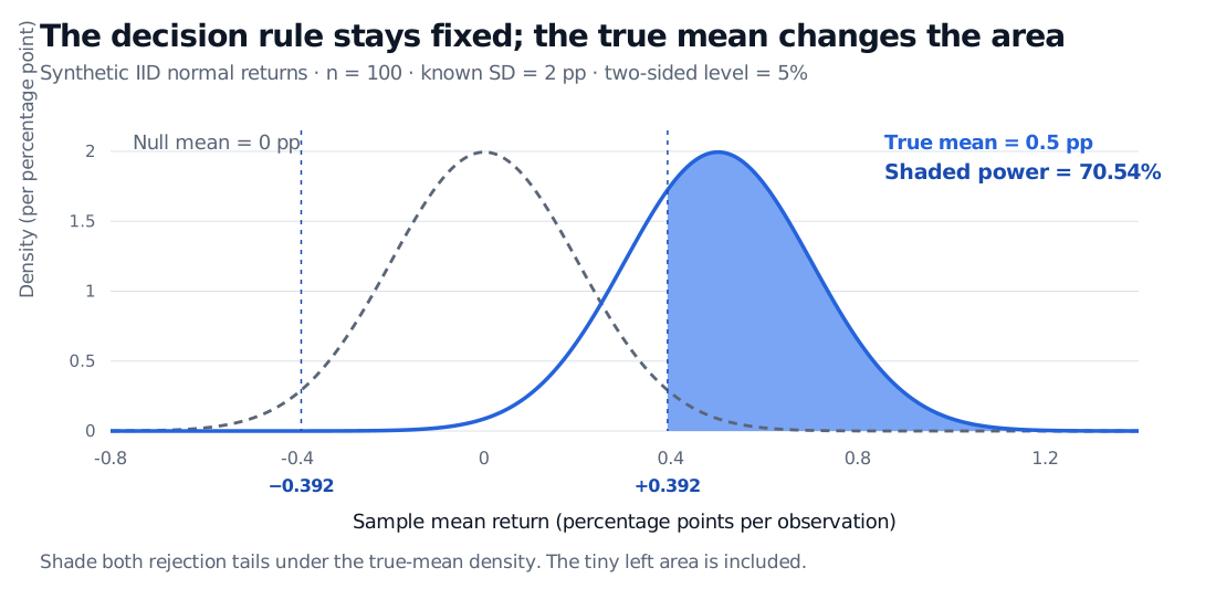
Now suppose the true mean is

\mu=0.5

percentage points. The statistic is no longer centred at zero:

Z\sim\mathcal{N}(2.5,1)

. We must calculate how much of this alternative distribution falls beyond the original cutoffs.

Sample-mean null and alternative normal densities for n 100 and known SD 2 percentage points. Fixed rejection cutoffs are minus and plus 0.392 percentage points. Shading under the alternative mean 0.5 distribution gives 70.54% power, including a tiny left tail.

Original model-based illustration. The shaded area belongs to the alternative distribution; its boundary comes from the null. Both distributions have sample-mean SD 0.2 percentage points.

For a general true mean, let

d=\sqrt n\,\mu/\sigma

. With

\Phi

denoting the standard normal distribution CDF, the exact two-sided power is

\begin{aligned} \pi(\mu) &=\mathbb{P}_{\mu}(Z<-c)+\mathbb{P}_{\mu}(Z>c)\\ &=\Phi(-c-d)+\Phi(d-c). \end{aligned}

d=2.5

, the lower-tail probability is approximately

0.000004099

and the upper-tail probability is

0.705413902

. Their sum is

0.705418001

: 70.54% power, leaving a 29.46% probability of failing to reject despite this genuine positive mean.

The small lower tail is included because this is a two-sided test of departure from zero. A rejection in the negative direction would not support a claim of positive expected return. A test designed specifically for a positive mean uses a different, predeclared one-sided rule.

The design determines what the test can see

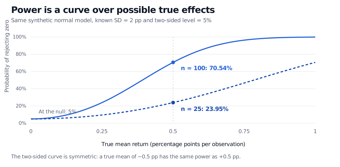
With only

n=25

, standard error doubles to

0.4

percentage points, the critical sample mean becomes

\pm0.7839856

percentage points, and the same true mean gives a shift of only

1.25

standard errors. Power falls to 23.95%. Both designs still have a 5% false-rejection probability at zero.

Two-sided power curves for known population SD 2 percentage points and level 5%. At true mean 0.5 percentage points, n 25 has 23.95% power and n 100 has 70.54% power. Both curves start at 5% rejection probability at true mean zero; negative effects have symmetric power.

Original normal-model calculations. The horizontal axis is a possible true mean, not an observed sample estimate. Solid: 100 observations; dashed: 25 observations. At zero, the plotted rejection probability is the false-alarm rate.

For this model, detection improves as the absolute effect size

|\mu|/\sigma

or the sample size grows. A stricter significance level moves the cutoffs outward and reduces power at a fixed alternative. These trade-offs should be evaluated against effects worth detecting before collecting data; NIST's sample-size guidance makes the desired shift, noise and error rates explicit planning inputs.

More rows help only to the extent that the model's information calculation remains valid. Overlapping returns, serial dependence, unstable means and changing strategies can invalidate the IID calculation. When population SD is estimated from the same normal sample, the exact mean test uses a Student $t$ statistic; its power requires a noncentral $t$ distribution under the alternative. Substituting an estimated SD into this known-SD formula does not preserve exactness.

Read the completed study differently

Power is a repeated-sampling probability conditional on a specified truth. It is neither the probability that the null is false after seeing data nor a probability that the strategy will make money. A 70.54% design does not assign a 70.54% probability of a genuine edge to the eventual backtest.

Nor should a researcher plug the observed sample mean into the true-mean input and report “observed power” as fresh evidence. For this fixed known-SD test, that calculation is determined by the absolute observed statistic, just as the two-sided p-value is; it adds no independent information. Hoenig and Heisey explain why this retrospective interpretation fails. After collecting data, report the estimated effect and its confidence interval, with the test's assumptions and any research selection made explicit.

Finally, adequate power for one predeclared test does not control false discoveries across a search through many strategies. Multiple hypothesis testing changes the decision procedure and therefore its power. A sensible study evaluates detection and false alarms together, for the procedure it will actually use.

For the interval calculations, normal-family testing assumptions and a return-history power example, continue with Confidence Intervals and Hypothesis Testing (membership; public preview).

Sources

Larry Wasserman, All of Statistics: A Concise Course in Statistical Inference, Chapter 10, Definition 10.1 and Example 10.2, pp. 150–152: power functions, test size and known-SD normal-mean testing. Author's book page.
NIST/SEMATECH e-Handbook of Statistical Methods, §7.2.2.2, “Sample sizes required”: effect, noise and error-rate inputs to study planning.
John M. Hoenig and Dennis M. Heisey (2001), “The Abuse of Power: The Pervasive Fallacy of Power Calculations for Data Analysis”, The American Statistician, 55(1), 19–24: the limitations of observed-power interpretations.

Fix the rule, then change the truth

A real edge can still produce an inconclusive history

The design determines what the test can see

Read the completed study differently

Sources

Related terms

Alternative hypothesis

Confidence interval

Hypothesis test

Normal distribution

Null hypothesis

P-value

Sample size

Standard error