Sample size counts observations, but precision depends on what is counted and how data arise. Plan a normal-mean interval, round correctly, and distinguish precision from power and effective information.
Sample size
Sample size, usually written n, is the number of observational units in a sample. The unit must be stated: days of a strategy's return history, independently simulated paths, audited orders or distinct firms. A million quote messages and a million independent trading days are different sources of information.
For a quant researcher, the useful question is not simply “Is n large?” It is “Does this sampling design provide enough information for this estimate or decision?” A mean, a tail quantile and a probability of a rare loss need different planning calculations.
More data buys precision at a decreasing rate
For independent, identically distributed observations with finite population variance σ2, the sample mean has
Var(Xˉ)=nσ2,SE(Xˉ)=nσ.
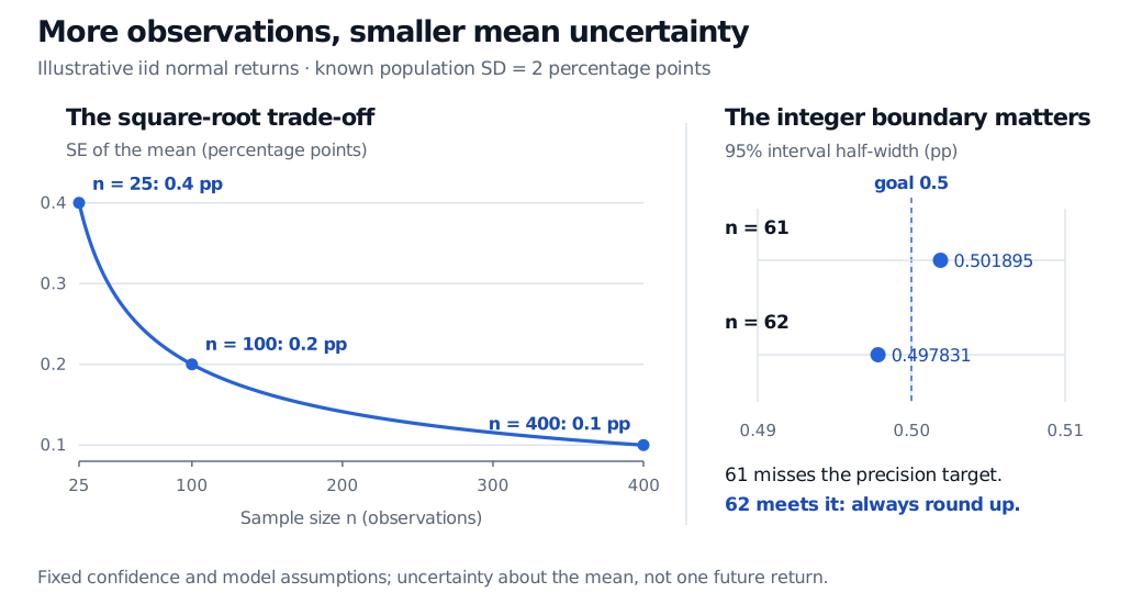
The standard error measures the mean's variation across repeated samples. It is different from the standard deviation of one return. With population SD fixed at 2 percentage points (pp), the mean SE is 0.4 pp at n=25, 0.2 pp at n=100 and 0.1 pp at n=400. Four times the observations halves the SE under this model; doubling the observations does not halve it. Rice derives this square-root relationship in §7.3.
None of this removes sampling bias. Repeatedly observing only surviving funds can estimate the survivor population's mean very precisely while missing the intended population of all funds. More observations from the same selected source do not repair that target mismatch.
Plan the width before collecting data
Suppose a research team wants to estimate the mean one-period return of a fixed hypothetical strategy. For this planning example, assume observations are iid normal, with unknown mean μ and known population SD σ=2 pp. Choose a fixed two-sided 95% confidence interval, and require its half-width to be at most h=0.5 pp. These are model assumptions and design choices, not facts established by a short return history.
The interval is
Xˉ±z0.975nσ,z0.975=Φ−1(0.975)≈1.959964.
Its half-width is deterministic here because σ is known. Solving the precision requirement gives
The ceiling symbol means round up. At n=61 the half-width is approximately 0.501895 pp, exceeding the target; at n=62 it is approximately 0.497831 pp. Rounding the unrounded requirement to the nearest integer would fail the design. The full desired interval width is 1 pp; using that full width in place of the half-width would solve a different problem.
Illustrative iid normal returns with known population SD 2 percentage points. Mean standard errors at sample sizes 25, 100 and 400 are 0.4, 0.2 and 0.1 percentage points. The 95% interval half-width is 0.501895 pp for n 61 and 0.497831 pp for n 62; 62 is the minimum integer meeting a 0.5 pp goal.
Original model-based calculations, not observed market data. Left: quadrupling n halves mean SE. Right: a magnified half-width scale shows why the required sample size must be rounded up. Confidence level and known population SD are fixed.
The 95% describes repeated-sampling coverage of the interval procedure. It does not promise that every realised sample mean is within 0.5 pp of the truth, nor does it put a 95% frequentist probability on a fixed mean after the interval is observed. NIST's normal-mean interval discussion makes the sampling interpretation explicit.
In practice, population volatility is usually unknown. A normal-model interval then uses a sample standard deviation and a Student t critical value. Both the future SD estimate and the critical value's dependence on n matter for width planning. Substituting a pilot SD into the known-SD formula is a planning approximation, not a guarantee that the eventual interval meets the target.
Precision, power and a valid stopping rule
A precision target asks how tightly a parameter will be estimated. Statistical power asks how often a prespecified hypothesis test rejects at a particular true alternative. Power planning additionally needs an effect size worth detecting, the alternative's direction and a target rejection probability. The 62-observation width calculation does not guarantee high power to detect an arbitrarily small positive mean. NIST treats precision and power as separate sample-size design problems in §7.2.2.2.
The calculation also assumes a fixed analysis. Collecting more returns whenever the result is disappointing, repeatedly inspecting conventional intervals and stopping when one excludes zero changes the procedure. Its fixed-sample coverage or error-rate claim need not survive that stopping rule. Specify the stopping and analysis rules beforehand, or use an inference method valid for the intended sequential design. Choosing the best-looking strategy after comparing many candidates is a separate selection problem, even when each candidate has many observations.
Count rows, then examine information
With dependent returns, covariance terms enter the mean's variance:
Var(Xˉ)=n21(i=1∑nVar(Xi)+2i<j∑Cov(Xi,Xj)).
Overlapping return windows or clustered executions can therefore make a large row count overstate the precision suggested by the iid formula. Dependence does not always inflate this variance: covariance signs and the estimator matter. Volatility clustering can violate independence even when return-level covariances are zero.
An effective sample size expresses information relative to a specified independent-sampling benchmark. It is not a universal corrected row count. It can differ across estimators and cannot by itself establish a valid confidence interval. Conversely, simple random sampling without replacement from a finite population can reduce mean variance through a finite-population correction.
There is no universal “n=30 is enough” rule. Exact normal-mean inference rests on its model; a central limit theorem approximation can converge slowly with heavy tails; rare-event estimation depends on how much relevant tail information the sample contains. A longer history may also span different regimes, so gaining rows can change the population question. Report the unit, inclusion rules, dependence assumptions and analysis design alongside n.
John A. Rice, Mathematical Statistics and Data Analysis, 3rd edition (2007), §7.3 (mean variance and sampling dependence), §7.3.3 (confidence intervals and width planning), §9.2 (power), and §9.5 (fixed-sample-size assumption).