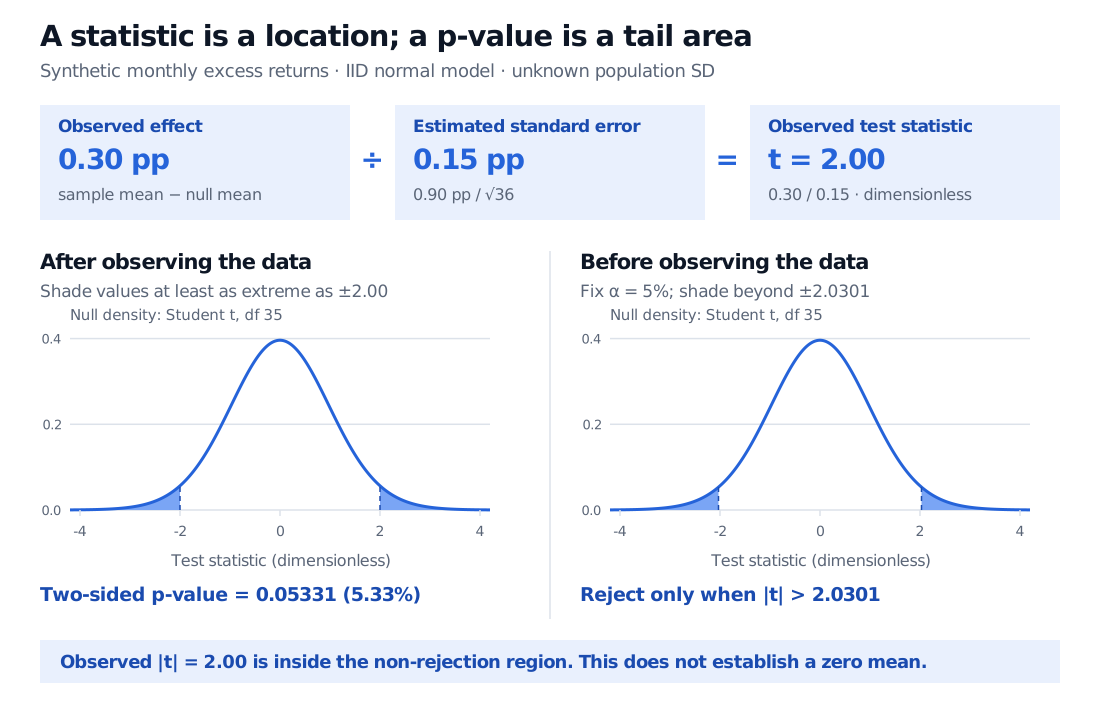
A test statistic maps sample data to evidence against a null. See how a return t value of 2 differs from its standard error, p-value and critical cutoff.
Test statistic
A test statistic is a function of sample data used to assess a null hypothesis. It compresses the evidence relevant to a specified test into a quantity whose behaviour under the null can be studied. The observed statistic is a number; its null reference distribution tells us which numbers would be unusual if the null and the sampling assumptions held.
A strategy's positive average return is an effect estimate. Whether that estimate is unusually far from zero depends on its uncertainty. A test statistic can put the two on a common scale, but the statistic alone does not supply a probability or a trading decision.
From a return estimate to a test statistic
Consider an original hypothetical strategy with 36 monthly excess-return observations. Before examining the results, the researcher specifies a two-sided hypothesis test of zero population mean, at a 5% significance level. For this example only, assume the observations are independent and identically distributed normal variables with unknown, positive population standard deviation.
Distance from the null in estimated standard-error units
The statistic is the rule
T(X1,…,Xn)=S/nXˉ−μ0,S2=n−11i=1∑n(Xi−Xˉ)2.
Here μ0=0, so the realised value is
tobs=0.90/360.30−0=0.150.30=2.
Uppercase T refers to the random statistic before sampling; lowercase tobs denotes the result calculated from this sample. Both numerator and denominator use percentage points, so the ratio is dimensionless. Expressing the returns as decimals instead gives 0.003/(0.009/6)=2.
The meaning of 2 is therefore “two estimated standard errors above the hypothesised mean.” It is neither a 2% return nor a 2% probability.
The reference distribution does a different job
Under the stipulated normal sampling model and the null μ=μ0,
T∼tn−1=t35.
This exact Student's t distribution accounts for estimating the population dispersion from the same sample. In the normal model, the standardised sample mean is normal and independent of the appropriately scaled sample variance, which has a chi-squared distribution. Their ratio produces the t law. Merely dividing an estimate by an estimated standard error does not automatically produce a standard-normal statistic—or an exact t statistic under arbitrary data.
For a two-sided alternative, values far from zero in either direction count as extreme. The p-value is therefore
p=PH0(∣T∣≥∣tobs∣)=2[1−Ft35(2)]≈0.05331,
where Ft35 is the null cumulative distribution function. This is a tail probability computed from the observed statistic and the reference law. It is not the probability that the zero-mean hypothesis is true.
The critical value answers a separate design question. With a predeclared two-sided significance level of α=0.05, choose the cutoff c so that the two null rejection tails total 5%:
c=Ft35−1(0.975)≈2.0301,reject if ∣tobs∣>c.
The observed value 2 falls short of 2.0301, and its p-value exceeds 0.05. The test therefore fails to reject zero mean at 5%. That result does not establish that the true mean is zero, nor that the strategy lacks economic value.
Synthetic IID normal monthly returns with n 36, mean 0.30 percentage points and sample SD 0.90. Estimated standard error is 0.15 and observed t is 2. Two null-density panels distinguish the observed two-sided tail area 0.05331 from the fixed 5% rejection tails beyond absolute t 2.0301.
Original hypothetical example. Both curves use Student t with 35 degrees of freedom. Shading covers both tails; the plotted horizontal range truncates their visual extent, while the reported probabilities include the full tails.
Why “t above two” is an incomplete research rule
Using a standard-normal reference at the same numerical value 2 would give a two-sided p-value of about 0.04550, crossing the 5% threshold. That would be a different reference calculation. It is exact for a normal mean with known population standard deviation when the denominator uses that known value; it cannot simply replace the t law in this unknown-dispersion example. Approximation error can matter near a decision boundary.
Actual return histories require a further check. Serial dependence can invalidate S/n as the standard error of the mean. Non-normal returns remove the exact finite-sample t guarantee; suitable large-sample approximations need their own conditions, and heavy tails can make them unreliable. A dependence-aware standard error changes the statistic, while its reference approximation must also be justified. Searching many strategies or choosing the test's direction after seeing the result introduces multiple-testing and selection issues that a lone t value cannot resolve.
The term test statistic is broader than this example: a raw count, a variance ratio or a likelihood ratio may serve the same role in another test. Each needs its own reference law and rule for which values count as evidence against the null. Report the statistic alongside the model, sample size, uncertainty estimate, alternative, p-value and effect size.
For the normal-family derivation and the connection to confidence intervals, continue with Confidence Intervals and Hypothesis Testing. The public preview gives the outline; the full lesson requires membership.
Sources
George Casella and Roger L. Berger, Statistical Inference, 2nd edition, §8.1, especially the test-statistic discussion after Definition 8.1.3; §5.3.2, Definition 5.3.4, for the normal-sample t construction.