Student's t-distribution: Definition & Examples

Student's t-distribution is a symmetric, bell-shaped family with heavier tails than the standard normal distribution. Its parameter

\nu>0

, called the degrees of freedom, controls tail thickness: smaller

\nu

means more probability far from the centre; as

\nu\to\infty

, the standard t law approaches

\mathcal N(0,1)

It has two distinct financial uses. As a reference distribution, it accounts for estimating an unknown standard deviation when testing a normal population mean. As a model for observations, a shifted and scaled t law can describe symmetric, heavy-tailed returns or P&L. These are different claims: a t-distributed test statistic does not mean that the underlying returns are t-distributed.

Where the extra tails come from

Let

Z\sim\mathcal N(0,1)

and

U\sim\chi^2_\nu

be independent, where

\chi^2_\nu

denotes the chi-squared distribution. Then

T=\frac{Z}{\sqrt{U/\nu}}\sim t_\nu.

A small random denominator can turn a moderate normal numerator into an extreme ratio. Increasing $\nu$ concentrates $U/\nu$ around one, reducing this extra source of variation. Independence is part of the construction; a ratio of arbitrarily related normal and chi-squared variables need not have this law.

The standard density is

f_\nu(t)=\frac{\Gamma((\nu+1)/2)}{\sqrt{\nu\pi}\,\Gamma(\nu/2)} \left(1+\frac{t^2}{\nu}\right)^{-(\nu+1)/2}, \qquad -\infty<t<\infty,

where

\Gamma

is the gamma function. Its tails decay as a power of

|t|

, rather than at the normal density's exponential-of-a-square rate. The family permits positive real degrees of freedom; integer

\nu=n-1

arises in the particular one-sample setting below. NIST's distribution reference illustrates the shape and normal limit; SciPy's mathematical definition specifies the positive-real parameter domain.

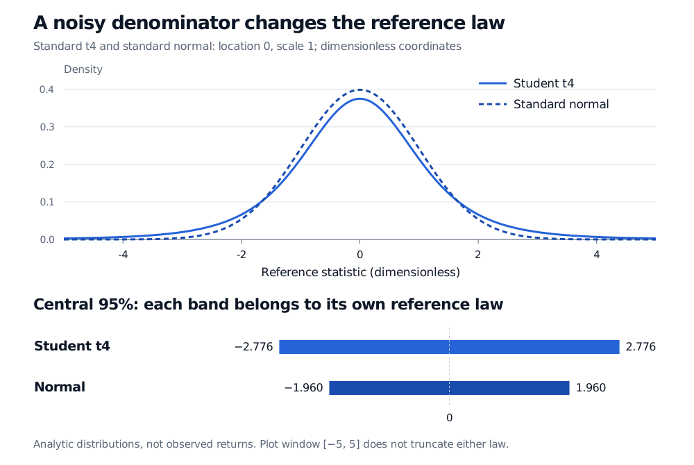
Standard t4 and standard normal densities, both with location zero and scale one. The central 95% interval is from minus 2.776 to plus 2.776 for t4, compared with minus 1.960 to plus 1.960 for the normal.

Original analytic comparison, with dimensionless axes. The two laws have equal location and scale, but different variances: t4 has variance 2 and the standard normal has variance 1. Display limits do not truncate either distribution.

Five observations are a short track record

Suppose a researcher has five synthetic, same-horizon strategy returns. For this example, assume the observations are independent draws from one normal distribution, with unknown mean

\mu

and unknown positive standard deviation

\sigma

. This is a stipulated teaching model, not an empirical claim about market returns.

Write

\bar X=\frac1n\sum_{i=1}^nX_i, \qquad S^2=\frac1{n-1}\sum_{i=1}^n(X_i-\bar X)^2.

Under this model,

\bar X

and

S^2

are independent, the standardised mean is normal, and

(n-1)S^2/\sigma^2\sim\chi^2_{n-1}

. Combining those results gives the exact sampling distribution

\frac{\bar X-\mu}{S/\sqrt n}\sim t_{n-1}.

The denominator is an estimated standard error, rather than the population standard deviation. One residual degree of freedom is lost because the observations were centred on the estimated mean.

Suppose the observed mean return is

\bar x=0.02

and the sample standard deviation is

s=0.04

: 2% and 4 percentage points respectively, over the stated observation horizon. For a predeclared two-sided test of

H_0:\mu=0

t_{\text{obs}}=\frac{0.02}{0.04/\sqrt5}=1.118034, \qquad \nu=4.

Quantity	Result under the stated normal-sampling model
Estimated standard error	$0.017889$ , or 1.7889 percentage points
Two-sided p-value	$\mathbb P(
Central 95% t cutoff	$t_{4,0.975}=2.776445$
95% interval for the mean	$0.02\pm2.776445(0.04/\sqrt5)$ , approximately $[-0.029667,\ 0.069667]$

Here

t_{4,0.975}

means the lower-CDF 97.5th percentile. Its two excluded tails total 5%. The observed statistic is inside the central region, so this test does not reject zero at the 5% level. The confidence interval includes zero and spans roughly −2.97% to +6.97% mean return per observation period.

The normal cutoff 1.96 would understate uncertainty in this exact unknown-variance problem. Conversely, 0.326164 is not the probability that the null is true, and failing to reject does not establish that the strategy has no economic value. The p-value describes repetitions of the statistic under the specified null model.

For the inference argument and its limits, Confidence Intervals and Hypothesis Testing develops the normal-family result and separates significance from trading value. Pivotal Quantities and Exact Confidence Intervals shows how inverting the same statistic produces the interval. Both offer public previews; full lessons require membership.

Scale is not standard deviation

For modelling an observation, write $Y=m+aT_\nu$ , with location $m$ and positive scale $a$ . Its density is $f_\nu((y-m)/a)/a$ . Location and scale have the units of $Y$ ; $\nu$ is dimensionless. This is a location-scale t distribution, not the separate noncentral t family.

Moment existence matters before using familiar risk summaries:

Degrees of freedom	Mean and variance
$0<\nu\le1$	Mean undefined; usual variance about the mean undefined
$1<\nu\le2$	Mean $m$ exists; variance is infinite
$\nu>2$	Mean $m$ ; variance $a^2\nu/(\nu-2)$

Thus, for $\nu>2$ ,

\operatorname{SD}(Y)=a\sqrt{\frac{\nu}{\nu-2}}.

A t4 return model with scale 4 percentage points has standard deviation $4\sqrt2\approx5.657$ percentage points. The sample standard deviation of 4 percentage points in the earlier inference example was a different object. To specify a t4 model with a desired standard deviation, divide that desired value by $\sqrt2$ to obtain its scale.

\nu=1

, the law is Cauchy: symmetry and a finite median do not give it a mean. More generally, a positive absolute moment of order

r

is finite exactly when

r<\nu

. In particular, t4 has finite variance but no finite fourth moment. A finite dataset's computed variance or kurtosis does not establish that its proposed population model has those moments.

Using a t return model also does not make the usual mean statistic exactly t-distributed: that exact inference result required normal observations. Serial dependence, changing volatility, selection among strategies and non-normal tails require their own justification or methods. A single symmetric marginal t law supplies neither return dynamics nor cross-asset dependence, and its unbounded support can conflict with a limited-liability simple-return model. Tail thickness is a modelling choice to assess, not an automatic correction for every backtest problem.

Sources

John A. Rice, Mathematical Statistics and Data Analysis, 3rd ed., §6.2, Proposition A, and §6.3, Theorem B and Corollary B, pp. 192–198: t construction, density and exact normal-sample pivot.
NIST/SEMATECH, e-Handbook of Statistical Methods, §1.3.6.6.4, “t Distribution”: distribution shapes, normal limit and special cases.
SciPy, scipy.stats.t: positive-real degrees of freedom, density, location-scale convention and distribution functions.

Where the extra tails come from

Five observations are a short track record

Scale is not standard deviation

Sources

Related terms

Cauchy distribution

Chi-squared distribution

Confidence interval

Independence

Normal distribution

P-value

Probability density function

Sample standard deviation

Sampling distribution

Standard error