A symmetric heavy-tailed distribution with a median and quantiles but no mean or variance. See why IID Cauchy averages retain the original scale and what that means for risk models.
Cauchy distribution
The Cauchy distribution is a continuous probability distribution with a location parameter m and a positive scale parameter s. It is symmetric and bell-shaped, but its tails are so heavy that its mean and variance are undefined. The location is its median, not an expected value, and its scale is not a standard deviation.
For a quant, the useful warning is concrete: even independent observations need not produce an average that becomes more concentrated as the sample grows. Cauchy observations provide an exact counterexample to applying familiar averaging rules without checking their assumptions.
These formulas still give valid probabilities and quantiles when moments do not exist. In particular, the lower and upper quartiles are m−s and m+s. The interquartile range is 2s: a useful interpretation of scale that does not rely on variance. The density has units reciprocal to X; its height at one point is not a probability.
A synthetic P&L model
Suppose a desk uses X∼Cauchy(0,2), in USD, as a deliberately extreme one-period P&L model for testing a risk calculation. This is a stipulated model, not a fitted distribution of trading results.
Its median is USD 0, and its quartiles are USD −2 and USD 2:
FX(−2)=41,FX(2)=43,P(−2≤X≤2)=21.
Thus half the probability lies within USD 2 of the centre. This does not say that USD 2 is a one-standard-deviation move: no population standard deviation exists. Since the distribution is continuous, including or excluding the interval endpoints does not change its probability.
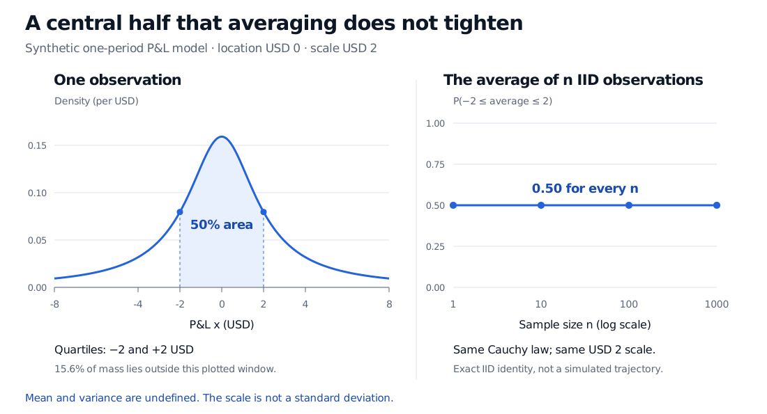
Analytic synthetic Cauchy P&L model with location USD 0 and scale USD 2. Density area between USD −2 and USD 2 is 50%; 15.6% lies outside the plotted USD −8 to USD 8 window. For IID averages with sample sizes 1, 10, 100 and 1000, the probability of remaining between USD −2 and USD 2 stays at 0.50.
Original analytic illustration. The finite density window is not renormalised. The right panel shows exact sampling probabilities, not a realised running average or observed market data.
Why symmetry does not give a mean of zero
For the model above, fX(x)=2/[π(4+x2)]. On the positive half-line,
∫0bxfX(x)dx=π1ln(1+4b2)⟶∞.
The negative half contributes −∞. An expected value cannot be obtained by cancelling these two divergent parts. Symmetric truncation does give
b→∞lim∫−bbxfX(x)dx=0,
but this is a Cauchy principal value, not the expectation. Consequently, the usual variance, defined around a population mean, is undefined too. The second raw moment E[X2] is infinite; that does not supply a missing mean or make the scale a volatility.
A finite set of realised Cauchy observations can still have an ordinary arithmetic average and sample variance. Calculating those numbers does not establish that the corresponding population moments exist. The Improper Integrals lesson develops the distinction between convergent integrals and symmetric cancellation. Its public page is a preview; the full lesson requires membership.
More independent observations do not narrow this average
If X1,…,Xn are independent and identically distributed Cauchy variables with location m and scale s, then
The sum's scale grows in direct proportion to n, so dividing by n leaves the average with the original distribution. For the synthetic desk model, P(∣Xˉn∣≤2)=1/2 for every positive integer n. Its sampling distribution never concentrates around zero.
One way to see the identity uses the characteristic function ϕX(t)=E[eitX]=eimt−s∣t∣. Independence gives
ϕXˉn(t)=[ϕX(t/n)]n=eimt−s∣t∣=ϕX(t).
This is consistent with the law of large numbers: the usual IID theorem requires a finite absolute first moment, which the Cauchy lacks. The standard finite-variance central limit theorem does not apply either. Independence alone supplies neither condition. The Weak Law lesson explains the finite-variance proof and the broader finite-mean result; it has a public preview and requires membership for the full lesson.
What this does—and does not—say about financial risk
Cauchy models are useful for stress-testing procedures that quietly require moments: mean-based forecasts, variance-based risk measures and conventional standard-error calculations. Quantiles remain meaningful, and a sample median can estimate the location even though a sample average fails to concentrate. More data can therefore help estimate the distribution; it is the averaging argument that fails here.
A heavy tail alone does not justify choosing a Cauchy law. Its exact symmetry and unbounded support impose strong assumptions. A fully paid cash position with limited downside cannot have an exact Cauchy P&L distribution, because the model assigns positive probability below every finite loss floor. Truncating the distribution changes its moments and destroys the exact averaging identity above. Choosing a tail model requires matching the position, horizon, support and evidence, rather than treating this counterexample as a forecast.
Joseph K. Blitzstein and Jessica Hwang, Introduction to Probability, 2nd edition, §7.1, Example 7.1.25: the Cauchy density from a ratio of independent standard normal variables and the failure of its expectation integral to converge.