A critical value is a boundary on a test statistic that separates rejection from non-rejection of a null hypothesis. It comes from the test's reference distribution and chosen significance level. The testing rule, including its tail direction and level, is specified before examining the results; the observed statistic is then compared with that boundary.
For a researcher testing a strategy's mean return, this turns “how far from zero is far enough?” into a defined rule. It does not turn statistical evidence into a guarantee of profitability.
Choose the tail before looking at the return
Write for the quantile of the standard normal distribution: the probability to its left is . If has this distribution under the null, the following rules have false-rejection probability :
| Alternative | Strict rejection rule | Cutoff at |
|---|---|---|
| Positive departure | ||
| Negative departure | ||
| Departure in either direction |
The two-sided rule allocates half the error budget to each tail. Using 1.645 in both tails would spend about 10%, rather than 5%. Choosing a positive one-sided test only after seeing a positive sample mean also changes the procedure; it does not preserve the advertised error rate. NIST's normal quantile table distinguishes the relevant quantiles.
Boundary convention. This article rejects only strictly beyond the critical boundary; equality means do not reject. For a continuous null distribution, equality has probability zero, so replacing a strict inequality with an inclusive one leaves the theoretical size unchanged. Still, software should document the rule and compare unrounded values. For these continuous tests, our convention corresponds to .
A 0.5% average crosses one boundary but not the other
Consider a hypothetical, fixed study of 100 daily excess returns. Assume independent, identically distributed normal returns, and suppose the population standard deviation is known to be 2 percentage points per day. The observed average is 0.5 percentage points per day. Test against .
The standard error is 0.2 percentage points, not 0.2% of the estimated mean. Under the stipulated null model, the statistic has a standard normal distribution exactly. NIST's one-mean testing guidance gives this known-standard-deviation construction.
| Two-sided level | Statistic boundaries | Equivalent sample-mean boundaries, percentage points per day | Result for the observed mean |
|---|---|---|---|
| 5% | Reject | ||
| 1% | Do not reject |
These raw-mean boundaries are centered on the null mean, zero. They are not confidence-interval endpoints centered on the observed mean.
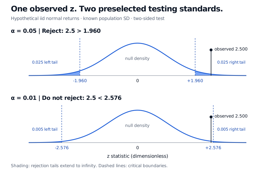
Original hypothetical normal-return calculation. Shaded rejection tails extend to infinity; the observed statistic stays fixed while the preselected significance level changes the boundaries.
The two-sided p-value is , consistent with both comparisons. This table compares two possible study designs; it is not permission to select the more convenient level after observing the result. Non-rejection at 1% does not establish that the true mean is zero.
Why 1.96 is not a universal hurdle
If the population standard deviation is estimated from these same normal observations, use
For , the two-sided 5% critical magnitude is , rather than 1.959964. The degrees of freedom matter; the numerical size of an estimated standard deviation does not make it a known population parameter. NIST's Student t table explains the degree-of-freedom and tail selections. Other statistics may require chi-squared, F, exact discrete or appropriately calibrated simulation reference laws.
In a discrete test, attainable tail probabilities jump. A nonrandomized rejection region may therefore have actual size below the nominal level; the boundary and whether its probability mass is included must be explicit. For a composite null, level control concerns the largest rejection probability over the null parameter set, not an arbitrary single null value.
A cutoff is only as credible as its reference model and research design. Dependent returns can invalidate the simple standard error; repeated backtest searches or repeated peeking can invalidate a single-test false-alarm claim. Tightening the boundary reduces false rejections but also reduces statistical power at a fixed alternative and sample size. Crossing it establishes neither economic value after costs nor the probability that the null is false.
For the derivation of the normal-family pivot and its matching confidence interval, read Confidence Intervals and Hypothesis Testing. A public preview is available; the full lesson requires membership.
Sources
- John A. Rice, Mathematical Statistics and Data Analysis, 3rd edition, §9.2, normal-mean threshold construction, and §9.2.1, specifying the significance level before analysis.
- NIST/SEMATECH: Standard Normal Cumulative Distribution Function, §1.3.6.7.1.
- NIST/SEMATECH: Critical Values of Student's t Distribution, §1.3.6.7.2.
- NIST/SEMATECH: Testing a Single Population Mean, §7.2.2.