F-distribution: Definition & Examples

The F-distribution is the probability distribution of a ratio of two independent chi-squared variables, each divided by its own degrees of freedom. It is a reference law for comparing estimated variances and for testing restrictions in normal linear models. A ratio is not F-distributed merely because both its numerator and denominator measure variation.

Let

U\sim\chi^2_{d_1}

and

V\sim\chi^2_{d_2}

be independent. Then

W=\frac{U/d_1}{V/d_2}\sim F_{d_1,d_2}.

The two parameters are ordered:

d_1

belongs to the numerator,

d_2

to the denominator. The chi-squared distribution explains the building blocks; the F law explains their relative size. Since both scaled quantities are dimensionless, so is

W

Why dividing by an estimate creates a long right tail

Each scaled chi-squared variable has mean one. Their ratio nevertheless does not generally have mean one: a small random denominator can produce a very large ratio. In particular, the expectation of a ratio is not the ratio of expectations.

For positive $d_1,d_2$ , the central F density is

f_W(w)= \frac{\Gamma((d_1+d_2)/2)}{\Gamma(d_1/2)\Gamma(d_2/2)} \left(\frac{d_1}{d_2}\right)^{d_1/2} \frac{w^{d_1/2-1}}{(1+d_1w/d_2)^{(d_1+d_2)/2}}, \qquad w>0.

Here $\Gamma$ is the gamma function. The variable is positive with probability one, has no point mass at zero, and has an unbounded right tail. Positive real degree parameters define the family; the interpretation as literal counts of independent squared standard normals applies to positive integers.

The first two moments are

\mathbb{E}[W]=\frac{d_2}{d_2-2},\qquad d_2>2,

\text{Var}(W)= \frac{2d_2^2(d_1+d_2-2)}{d_1(d_2-2)^2(d_2-4)}, \qquad d_2>4.

These are existence conditions, not suggestions about sample size. The mean diverges for

d_2\le2

; a finite variance requires

d_2>4

. For

F_{5,10}

, the mean is

1.25

and the variance is

65/48\approx1.354167

. Even under equal population variances, the expected sample-variance ratio can exceed one. The NIST F-distribution reference gives these distributional properties.

Two hedging rules, a fourfold variance ratio

Consider an original synthetic comparison of one-period P&L from two hedging rules, each applied to the same position size. Rule A has 6 observations; rule B has 11. Assume each sample is iid normal, the samples are independent of each other, and both population means are unknown. Independence could be imposed in a simulator through independent scenario streams; it should not be presumed for two rules exposed to the same market days.

Using the sample variance around each sample's own mean, with divisor

n_i-1

, suppose the observations give:

Quantity	Rule A	Rule B
Sample size	6	11
Sample variance	$0.04\ \text{USD}^2$	$0.01\ \text{USD}^2$
Sample standard deviation	USD 0.20	USD 0.10
Residual degrees of freedom	5	10

Before observing the samples, the team specifies the null hypothesis $H_0:\sigma_A^2=\sigma_B^2$ and the upper-sided alternative $H_1:\sigma_A^2>\sigma_B^2$ .

Normal-sample variance theory gives independent variables

U=\frac{5S_A^2}{\sigma_A^2}\sim\chi^2_5, \qquad V=\frac{10S_B^2}{\sigma_B^2}\sim\chi^2_{10}.

Under the null, the common population variance cancels:

\frac{U/5}{V/10}=\frac{S_A^2}{S_B^2}\sim F_{5,10}, \qquad w_{\mathrm{observed}}=\frac{0.04}{0.01}=4.

Both the USD-squared units and the degrees-of-freedom factors cancel in the statistic. Do not multiply the sample-variance ratio by $10/5$ again. The 5 and 10 still determine its reference distribution.

The upper-sided p-value is

p=\mathbb{P}(F_{5,10}\ge4) =0.0296752952\ldots\approx2.97\%.

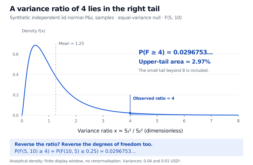
Synthetic independent iid normal P&L samples give sample variances 0.04 and 0.01 USD squared, an observed ratio of 4 and an F distribution with numerator 5 and denominator 10 degrees of freedom. The mean is 1.25. The shaded right-tail probability beyond 4 is 0.0296753, about 2.97%. Reversing the ratio gives 0.25 with degrees of freedom 10 and 5 and the same lower-tail probability.

Original analytical plot for the synthetic equal-variance null. The shaded probability includes the tail beyond the displayed range; the density is not renormalised. The blue dot marks the attained density value at the observed statistic.

At a prespecified 5% significance level, the upper-sided test rejects equal variances in the direction of higher variance for A. It does not say there is a 97.03% probability that A's population variance is higher. The probability describes repeated sampling under the null model, not uncertainty about which hypothesis is true.

The question's direction matters. For an equal-tail two-sided test of unequal variances, the p-value here is

2\min\{\mathbb{P}(F_{5,10}\le4),\mathbb{P}(F_{5,10}\ge4)\} =0.0593505904\ldots.

That test does not reject at 5%. Choosing the upper-sided question after seeing that A has the larger sample variance changes the procedure; it does not preserve the advertised one-sided error rate. NIST distinguishes the upper, lower and two-sided variance tests.

Keep the order; check the model

Taking the reciprocal swaps the degree parameters:

W\sim F_{d_1,d_2}\quad\Longrightarrow\quad \frac1W\sim F_{d_2,d_1}.

Thus

\mathbb{P}(F_{5,10}\ge4)=\mathbb{P}(F_{10,5}\le0.25)

. Reversing the ratio while keeping

F_{5,10}

would answer the wrong question. More generally, when population variances differ, the normalised ratio

\frac{S_A^2/\sigma_A^2}{S_B^2/\sigma_B^2}\sim F_{5,10}

still has the F law under the stated sampling assumptions. The raw sample-variance ratio then has an additional population-variance scale factor.

An observed fourfold variance ratio means a twofold sample standard-deviation ratio, not fourfold volatility. Nor does the exact calculation automatically carry over to heavy-tailed, serially dependent or changing-volatility market P&L. A large sample alone does not make the unadjusted normal-theory variance-ratio test valid. The variance comparison also says nothing directly about mean returns or hedge bias.

The same central family appears in linear regression, where independent normal-model sums of squares compare explained variation with residual noise under the null. A useful link is

T^2\sim F_{1,\nu}

when

T

has a central Student's t-distribution with

\nu

degrees of freedom. Squaring discards the sign, so this F test corresponds to a two-sided t test. Regression F statistics under alternatives can instead have a noncentral F law; “F statistic” does not guarantee the central null distribution everywhere.

For the construction and t-squared identity, read The Chi-Squared, t, and F Distributions. The ANOVA F-Test and R² develops the regression sum-of-squares application. Both full lessons require membership; public previews are available.

Sources

John A. Rice, Mathematical Statistics and Data Analysis, 3rd ed., §6.2, definition and Proposition B, and §6.3, Theorem B — F construction, density, t-squared relationship and normal-sample variance law.
NIST/SEMATECH e-Handbook: F Distribution — density and moment conditions.
NIST/SEMATECH e-Handbook: F-Test for Equality of Two Variances — ordered degree counts and one-sided versus two-sided alternatives.

Why dividing by an estimate creates a long right tail

Two hedging rules, a fourfold variance ratio

Keep the order; check the model

Sources

Related terms

Chi-squared distribution

Expected value

Independence

Linear regression

Normal distribution

P-value

Sample variance

Student's t-distribution