Multiple linear regression: Definition & Examples

Multiple linear regression models one response using two or more predictor columns, with a separate coefficient for each. In a financial factor regression, the response might be a fund's excess return, while the predictors describe market returns, other factor returns or observable scores. Fitting them together estimates each predictor's association with the response after adjusting for the others.

This changes the question asked by linear regression: instead of asking how fund returns move with the market alone, a researcher can ask how they move with the market given the other included exposures. Adding controls does not, by itself, turn that association into a causal effect.

One response, several slopes

With $n$ observations and $k$ predictor columns, write

y_i=\beta_0+\sum_{j=1}^{k}\beta_jx_{ij}+\varepsilon_i, \qquad i=1,\ldots,n.

The intercept is

\beta_0

;

\varepsilon_i

is the unobserved disturbance. A fitted residual,

e_i=y_i-\hat y_i

, is the observed discrepancy after estimating the coefficients. These are different objects.

“Linear” refers to the coefficients. Squared predictors, log-transformed predictors and interaction columns can enter a linear regression when their coefficients enter additively. An interaction changes how a slope depends on the other variables, so a constant “holding everything else fixed” reading must then be adjusted. This flexibility is part of the NIST definition of linear least-squares models.

For the additive model above, increasing predictor

j

by one unit while fixing the other predictor values changes the fitted response by

\hat\beta_j

. That is a partial slope within the specified model. It need not equal the slope from regressing the response on that predictor alone. Other predictors may share the same variation, and the sample may contain little evidence about moving one while holding the others fixed.

Five months, a market return and a score

Consider these synthetic monthly observations. Market excess return

x

and fund excess return

y

are recorded as percent numbers:

2

means

2\%

. The second predictor

z

is a dimensionless score, not another return. All rows refer to the same month and use the same excess-return basis.

Month	Market $x$ (%)	Score $z$	Fund $y$ (%)	Fitted $\hat y$ (%)	Residual $e$ (pp)
1	−2	2	−1	−0.829	−0.171
2	−1	−1	0	−0.486	0.486
3	0	−2	0	0.429	−0.429
4	1	−1	2	1.914	0.086
5	2	2	4	3.971	0.029

Ordinary least squares chooses the coefficients to minimise the sum of squared residuals. The fitted equation here, in the displayed numerical units, is

\boxed{\hat y=1+\frac65x+\frac27z.}

The intercept is a monthly fund excess return of $1\%$ at $x=z=0$ . A one-percentage-point higher market return is associated with a $1.2$ pp higher fitted fund return, fixing the score. A one-unit higher score is associated with a $2/7$ pp higher fitted fund return, fixing market return. The intercept describes the model at zero predictors; it is not automatically evidence of investment skill.

For month 5, the exact fitted value and signed residual are

\hat y_5=1+\frac65(2)+\frac27(2)=\frac{139}{35}\%, \qquad e_5=4-\frac{139}{35}=\frac1{35}\text{ pp}.

The table rounds to three decimals; the calculations use exact values. If returns are instead entered as decimals, the intercept becomes

0.01

and the market coefficient stays

1.2

. Because the dimensionless score is unchanged, its coefficient becomes

\frac27\times0.01

in decimal-return units per score unit. Coefficient units follow the units of both response and predictor.

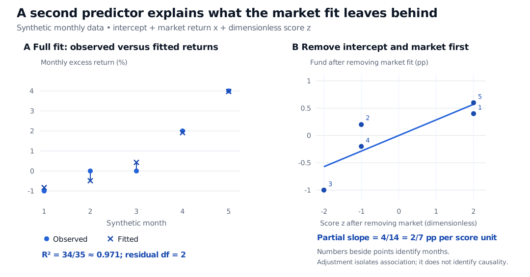
Five synthetic monthly fund returns and full fitted values, followed by a partial-regression plot. After removing intercept and market, fund values are 0.4, 0.2, −1, −0.2 and 0.6 pp. Regressing these against the dimensionless score gives slope 2/7 pp per unit; full-model R-squared is 34/35 with two residual degrees of freedom.

Original synthetic monthly example. Panel A shows observed and full fitted returns. Panel B removes the intercept and market from both fund return and score before examining the score's contribution; point labels identify months.

The partial-regression calculation explains “adjusting for market.” First regress $y$ on an intercept and $x$ , then retain the residuals $u_i$ . Separately regress $z$ on that same intercept and $x$ , retaining residuals $v_i$ . The score coefficient in the full model is

\hat\beta_z=\frac{\sum_i v_i u_i}{\sum_i v_i^2}.

Here both predictor columns are centred and $\sum_i x_i z_i=0$ , deliberately simplifying the example. The market-only fit is $1+1.2x$ , and its residuals are $(0.4,0.2,-1,-0.2,0.6)$ pp. Removing intercept and market leaves the score unchanged, so $v_i=z_i$ . Hence $\sum_i v_i u_i=4$ and $\sum_i v_i^2=14$ , giving $2/7$ . The market coefficient happens to remain unchanged when the score is added because these predictor columns are orthogonal. That is a feature of this constructed sample, not a general property of multiple regression.

What must the matrix tell you?

Put the intercept and predictors into the design matrix $X$ , with one observation per row. The fitting problem is

\hat{\boldsymbol\beta} =\operatorname*{arg\,min}_{\mathbf b}\lVert\mathbf y-X\mathbf b\rVert_2^2.

There are $k+1$ coefficients including the intercept. They are unique exactly when $X$ has full column rank. Merely having more observations than coefficients does not ensure that: a duplicated predictor, or a full set of category indicators alongside an intercept, can make a column redundant. With rank deficiency the OLS fitted vector remains unique, but the coefficient allocation need not be.

For this example,

X^\top X= \begin{pmatrix} 5&0&0\\ 0&10&0\\ 0&0&14 \end{pmatrix}.

Its three positive diagonal entries verify full column rank. The fitted residuals satisfy

X^\top\mathbf e=\mathbf0

: their sum is zero, and their inner product with each included predictor is zero. This is a property of the fit; it does not prove that the unobserved disturbances are exogenous.

Under full rank the familiar algebraic expression is

(X^\top X)^{-1}X^\top\mathbf y

. Compute the fit using QR or SVD rather than explicitly forming that inverse. R's lm documentation specifies QR fitting. The owned lesson Least Squares and Regression Geometry develops residual orthogonality and the numerical reason for preferring these factorizations (public preview; full lesson requires membership).

With nearly dependent predictors, the coefficients can be unstable even while the combined fitted returns look stable. This is the attribution problem behind multicollinearity: the data may identify a combined exposure more clearly than each separate loading.

A strong fit is only a beginning

For the five-month example, the centred total sum of squares is $\mathrm{SST}=16\text{ pp}^2$ and the residual sum is $\mathrm{SSE}=16/35\text{ pp}^2$ . Thus

R^2=1-\frac{\mathrm{SSE}}{\mathrm{SST}}=\frac{34}{35}\approx0.971.

This R-squared describes in-sample fit. Five rows minus three estimated coefficients leave only two residual degrees of freedom. The data are a transparent arithmetic example, not evidence that the score is useful in investment decisions. With the same response rows, adding predictors cannot lower ordinary OLS R-squared; adjusted R-squared accounts for parameter count but still does not measure future performance.

Computing these coefficients requires no normal-error assumption. Unbiasedness, standard errors, confidence intervals and tests require additional assumptions or an appropriate alternative inference framework. Changing volatility and serial dependence in financial returns can invalidate classical standard errors; robust covariance estimates do not repair omitted-variable bias or establish causality. The owned Regression Assumptions and Diagnostics separates those coefficient and inference problems (public preview; full lesson requires membership).

A contemporaneous factor fit also uses predictor values realised during the response month. Forecasting requires specifying which inputs were available at the forecast origin and evaluating on later data. For the full matrix derivation and conditional tests, continue to Multiple Linear Regression (public preview; full lesson requires membership); its exact finite-sample inference starts from explicitly normal, independent, constant-variance errors.

Sources

James, G., Witten, D., Hastie, T. and Tibshirani, R. (2021). An Introduction to Statistical Learning with Applications in R, 2nd edition, §3.2.1 (multiple-regression coefficients and interpretation) and §3.3.3, “Collinearity.”
NIST/SEMATECH e-Handbook, §4.1.4.1: Linear Least Squares Regression.
R stats documentation: lm — Fitting Linear Models.

One response, several slopes

Five months, a market return and a score

What must the matrix tell you?

A strong fit is only a beginning

Sources

Related terms

Adjusted R-squared

Coefficient of determination

Intercept

Linear regression

Ordinary least squares

Residual