Idiosyncratic risk is asset-specific uncertainty relative to a stated factor model. See how 25-stock diversification changes when residuals are correlated.
Idiosyncratic risk
Idiosyncratic risk is the uncertainty specific to an asset or issuer after accounting for the common risk factors in a stated model. It is also called specific risk or unsystematic risk. A company-specific product failure, fraud discovery or unexpectedly successful launch can move its shares even when the wider market barely changes.
The qualification “in a stated model” matters. In measured portfolio risk, idiosyncratic risk is usually represented by a residual. A market-only model leaves different things in that residual from a model that also includes industry, country and style factors. An unexplained return is not automatically an economically unique shock.
First remove the common exposure
A one-factor return model writes
Ri=αi+βiM+εi.
Here Ri and M are the stock and market returns over the same horizon, αi is a constant intercept, βi is the stock's market beta, and εi is its residual return. Assume finite variances, E[εi]=0 and Cov(M,εi)=0. Then
Var(Ri)=βi2Var(M)+Var(εi).
The first term is exposure to the specified common factor; the second is residual variance. Variances add here, not standard deviations. The zero-covariance condition removes the cross term. It does not establish independence, either between the market and a residual or between different stocks' residuals.
For example, a manufacturer's own production defect may primarily affect that firm. A surprise rise in financing costs may affect many firms together: that belongs to systematic risk, potentially represented by several common factors. If the manufacturer and its peers all depend on the same supplier, their apparently separate “company shocks” can have a common source that a market-only model misses.
An ordinary least-squares fit with an intercept makes fitted residuals orthogonal to its included regressors within the fitted sample. That property does not guarantee zero residual correlations across firms, stable exposures in the future, or an economically complete model. The single-index model adds the simplifying restriction that different firms' residuals are uncorrelated; merely estimating a market regression does not impose it.
What 25 equal holdings actually achieve
Consider a synthetic portfolio of 25 stocks, each with market beta 1. Use one-month simple returns in decimal units. The market's monthly standard deviation is 2%, and every stock's residual standard deviation is 3%. Residuals are uncorrelated with the market. Initially suppose the residuals are also pairwise uncorrelated across stocks. Intercepts do not affect these variance calculations.
For one stock,
Var(Ri)=0.022+0.032=0.0013,
so its monthly standard deviation is 3.6056%. Allocate equal initial weights, wi=1/25, and hold them over the month. The portfolio retains beta 1, while its residual variance becomes
Var(εP)=i=1∑25(251)20.032=250.0009=0.000036.
Its residual standard deviation is therefore 0.6%, and its total monthly standard deviation is
σP=0.0004+0.000036=0.0208806…≈2.0881%.
This is the mechanism of diversification: individual shocks receive smaller weights, while uncorrelated residual variances accumulate with squared weights. The portfolio still shares the market shock. Holding 25 names has reduced specific risk substantially; it has not made the portfolio safe from a market decline or even eliminated its residual risk.
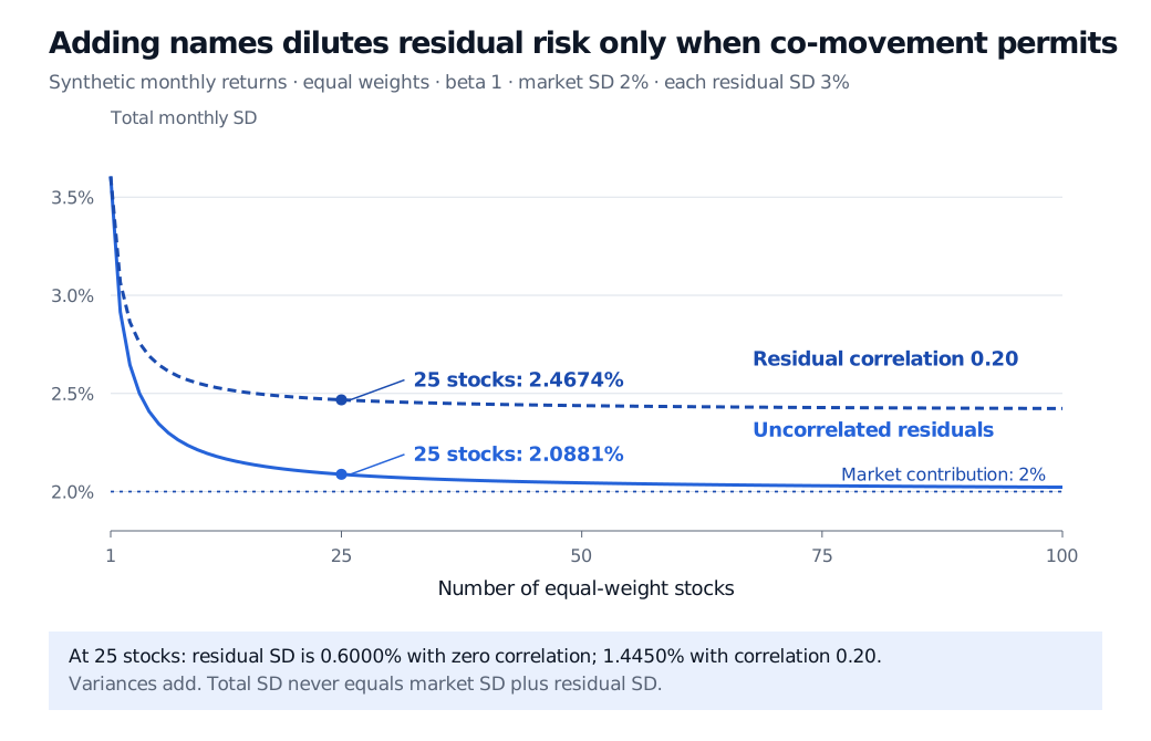
Synthetic monthly-risk curves: with market SD 2%, residual SD 3% and all betas 1, total SD falls from 3.6056% for one stock to 2.0881% for 25 equal holdings with uncorrelated residuals. Residual correlation 0.20 instead gives 2.4674% at 25 stocks. The market contribution remains 2%.
Original synthetic one-month model. Equal initial weights and unchanged beta; solid curve uses uncorrelated residuals, dashed curve uses residual correlation 0.20. The dotted 2% line is the unchanged market contribution to standard deviation.
When the residuals move together
Keep every input above, but give every distinct pair of residuals the same correlation, ρ=0.20. For N equally weighted stocks with common residual standard deviation σε,
Var(εP)=σε2(ρ+N1−ρ).
There are N diagonal variance terms and N(N−1) off-diagonal covariance terms in the full weighted sum. At 25 stocks this gives
With persistent positive residual correlation, increasing N does not remove the entire residual component: its variance approaches 0.0009×0.20=0.00018. Total monthly standard deviation approaches 2.4083%, above the 2% market contribution. This is a deliberately simplified correlation structure, not an estimate from market data. It demonstrates why treating every regression residual as fully diversifiable can understate portfolio risk. An omitted industry factor is one possible explanation for the co-movement.
Even with uncorrelated residuals, name count alone is insufficient. For unequal weights the residual term is ∑iwi2σεi2. A large position can dominate it. Diversification toward zero requires residual variances to remain controlled and weights to become sufficiently dispersed; more holdings with a dominant concentrated position do not supply that guarantee. Uncorrelatedness is also a second-moment property, so it does not establish independence of extreme losses.
What the label does—and does not—tell a manager
Specific-risk estimates help a manager distinguish a concentrated stock view from a broad factor bet, size issuer exposure and diagnose why portfolios with similar betas can have different volatility. For an employee whose salary and shares depend on one company, a firm-specific shock can be especially costly even if a diversified investor could dilute the same exposure.
The CAPM predicts no separate expected-return premium simply for bearing diversifiable specific risk, under its equilibrium assumptions. That is a model statement, not a promise that risky individual companies deliver poor or good realised returns. Nor does identifying a residual reveal stock-picking skill: omitted factors, estimation noise and changing business exposures all affect the result. CFA Institute's portfolio-risk reading places the pricing claim within the CAPM framework.
Finally, idiosyncratic, systematic and systemic describe different things. A firm-specific loss is idiosyncratic; exposure to shared return drivers is systematic; disruption that spreads through the financial system and impairs its functioning is systemic. A shock beginning at one institution can become systemic through contagion. The ECB's discussion of systemic risk explicitly allows a limited initial shock to trigger a wider systemic event.
For the portfolio-beta and variance derivation, continue with Sharpe's Single-Index Model. Its full lesson requires membership; the public page provides a preview.
Sources
Edwin J. Elton, Martin J. Gruber, Stephen J. Brown and William N. Goetzmann, Modern Portfolio Theory and Investment Analysis, 9th edition, 2014, Chapter 7, pp. 129–135: return decomposition, portfolio risk, Table 7.2 and footnote 7 on correlated residuals. The numerical examples and figure above are original.