Systematic risk: Definition & Examples

Systematic risk is the uncertainty associated with common sources of return variation that affect many assets. In an equity market model, it is the part linked to movements in a broad market index. Buying more stocks can spread company-specific surprises, but it does not remove a shared market exposure merely by increasing the number of holdings.

A retailer and a software company may have very different businesses yet both lose value when investors revise growth expectations or discount rates. The shared response is the systematic component. A warehouse fire or a failed product launch may instead create idiosyncratic risk. The distinction helps a portfolio manager ask whether a position adds another independent business risk or increases a bet the portfolio already carries.

Put the common exposure into an equation

A simple one-factor model for a stock's monthly simple return is

R_i=\alpha_i+\beta_i M+\varepsilon_i.

Here

M

is the monthly market-index return,

\alpha_i

is a constant intercept, market beta

\beta_i

is a dimensionless exposure, and

\varepsilon_i

is a zero-mean residual. Assume finite second moments and

\text{Cov}(M,\varepsilon_i)=0

. Then

\underbrace{\text{Var}(R_i)}_{\text{total variance}} = \underbrace{\beta_i^2\text{Var}(M)}_{\text{systematic variance}} + \underbrace{\text{Var}(\varepsilon_i)}_{\text{residual variance}}.

Without zero covariance, the expansion also contains

2\beta_i\text{Cov}(M,\varepsilon_i)

. The clean split depends on that condition. An ordinary least-squares regression with an intercept makes fitted residuals orthogonal to the market in the estimation sample; it does not prove that the relationship will hold in future data. Zero covariance also does not, by itself, establish independence.

Beta measures exposure rather than total volatility. A negative beta reverses the direction of the common response, but its squared contribution to standalone variance is still nonnegative. A zero market beta removes this one linear market component, while residual risk and exposure to omitted factors can remain.

One stock, then 25 stocks

Suppose a fictional stock has beta 1.5, monthly market standard deviation 2%, and monthly residual standard deviation 1%. Assume the market and residual are uncorrelated. Using decimal returns,

\begin{aligned} \text{Systematic variance}&=1.5^2(0.02)^2=0.0009,\\ \text{Residual variance}&=(0.01)^2=0.0001,\\ \text{Total variance}&=0.001,\\ \text{Total standard deviation}&=\sqrt{0.001}\approx3.1623\%. \end{aligned}

Thus 90% of the stock's variance is assigned to the market component in this model. Systematic standard deviation is 3% and residual standard deviation is 1%; these do not add to 4%. Variances add under the zero-covariance assumption, after which we take the square root. None of these inputs specifies an expected return.

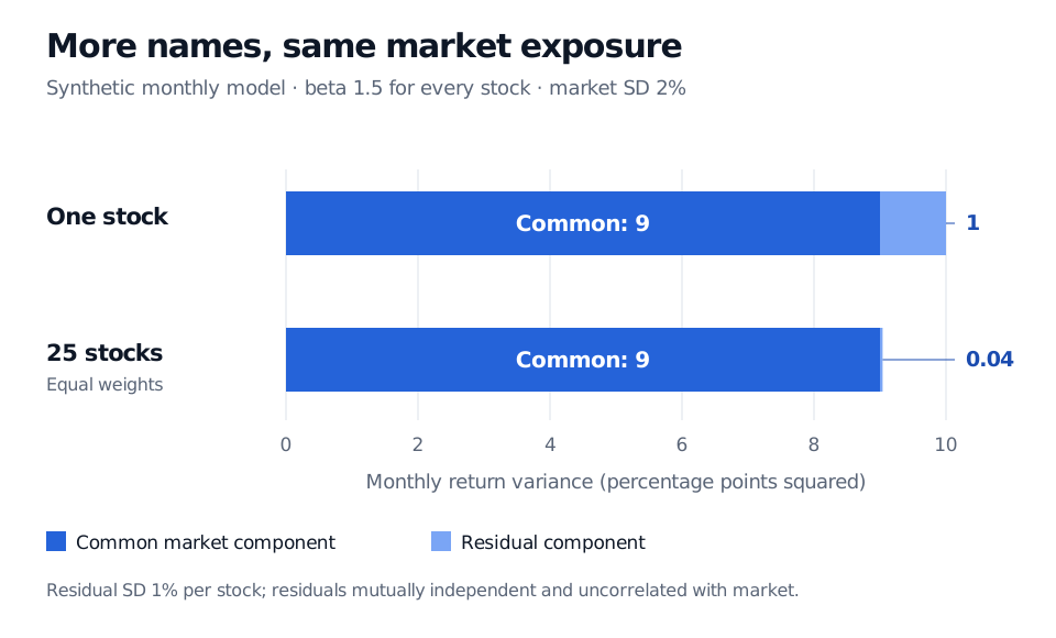
Now spread capital equally across 25 fictional stocks. Give each the same beta and residual standard deviation, and assume their residuals are mutually independent and each uncorrelated with the market. The portfolio still has beta 1.5. Its residual variance falls to

\text{Var}(\varepsilon_P) =\sum_{i=1}^{25}\left(\frac{1}{25}\right)^2(0.01)^2 =\frac{0.0001}{25}=0.000004.

Monthly risk measure	One stock	25 equal-weight stocks
Systematic variance, decimal-return squared	0.0009	0.0009
Residual variance, decimal-return squared	0.0001	0.000004
Total variance, decimal-return squared	0.001	0.000904
Total standard deviation	3.1623%	3.0067%

Synthetic monthly variance comparison: one stock has common variance 9 and residual variance 1 in percentage-point squared units; 25 equal-weight stocks retain common variance 9 while residual variance falls to 0.04. Each stock has beta 1.5, residual standard deviation 1%, and market standard deviation 2%; residuals are mutually independent and uncorrelated with the market.

Original synthetic one-factor model. Variance is shown in percentage points squared: multiply decimal-return variance by 10,000. The common component stays fixed because the portfolio's beta stays fixed.

This is why diversification can work well and still leave a portfolio exposed to a market decline. The 25-stock portfolio has much less residual variance, yet its total standard deviation remains close to 3% because the common component already dominates.

The reduction is conditional. Mutually uncorrelated residuals are sufficient for this variance calculation; independence is stronger than necessary. If many holdings share an omitted industry shock, their residual covariances need not be zero. Concentrated weights can also prevent risk from washing out. In the extreme case of identical residuals, adding more equal-weight names does not reduce residual variance at all.

“Systematic” depends on the model

A broad market index is one useful common factor, not a complete catalogue of economic uncertainty. An industry shock may sit in the residual of a market-only model but become an explicit common component when an industry factor is added. Changing the benchmark, return horizon or factor set can change the measured split.

In a multi-factor model with exposure vector $\mathbf b_i$ and factor covariance matrix $\Sigma_F$ , the common variance is $\mathbf b_i^\top\Sigma_F\mathbf b_i$ , assuming the residual is uncorrelated with every factor. Correlated factors contribute cross terms; adding their individual variance terms alone would miss them.

For a deeper treatment, Multi-Index and Mixed Models explains how industry and other factors capture co-movement missed by a single market index. The public page offers a preview; the full lesson requires membership.

Calling systematic risk “non-diversifiable” means it survives spreading holdings while retaining the common exposure. It does not mean the exposure is impossible to change. A portfolio can alter its factor loadings or use hedges, subject to trading costs, constraints, basis risk and model error. Nor does identifying a systematic component guarantee a risk premium. An asset-pricing model adds assumptions connecting exposures to expected returns; a covariance decomposition alone supplies neither that connection nor a return forecast.

Systematic and systemic are different questions

Systematic describes common return exposure. Systemic concerns disruption to the financial system's ability to provide services, with consequences for the wider economy. The BIS discussion of systemic risk emphasises interconnections, common exposures and spillovers beyond an individual institution.

The ideas can interact: a common asset-price shock may stress many leveraged institutions at once, and their responses may amplify it. But an ordinary broad market movement can generate systematic portfolio risk without causing systemic disruption. Conversely, trouble beginning at one institution can spread through financial connections. A stock's market beta does not measure that propagation mechanism.

Sources

Edwin J. Elton, Martin J. Gruber, Stephen J. Brown and William N. Goetzmann, Modern Portfolio Theory and Investment Analysis, 9th edition (Wiley, 2014), Chapter 7, especially “Single-Index Models: An Overview,” the variance derivation and diversification discussion; Chapter 8 on multi-index models. Numerical scenarios and the figure here are original.
Eric Zivot, Introduction to Computational Finance and Financial Econometrics with R, Chapter 16: Single Index Model, §16.2, explains shared factor exposure and the systematic/residual variance decomposition.
Bank for International Settlements, “Systemic risk: how to deal with it?”, 12 February 2010, distinguishes financial-service disruption and economy-wide spillovers from an individual investment loss.

Put the common exposure into an equation

One stock, then 25 stocks

“Systematic” depends on the model

Systematic and systemic are different questions

Sources

Related terms

Covariance

Diversification

Idiosyncratic risk

Market beta

Standard deviation

Volatility