The row space spans a matrix’s measurement directions. Use a three-instrument exposure example to distinguish column space, invisible holding changes and minimum-norm solutions.
Row space
The row space of a matrix is the set of all linear combinations of its rows. If A has m rows and n columns, each row has n coordinates, so its row space is a subspace of Rn.
For an exposure matrix whose columns are instruments, those coordinates refer to instruments. Each row tells a risk desk how one reported exposure changes with its holdings. The row space collects the exposure-measurement directions already represented by the matrix; adding a row inside that space adds no independent measurement.
Two reported factors, one independent exposure
Consider an original synthetic model of three instruments and two factor-exposure scores. Positions are measured in standardised instrument units, and every matrix entry is a dimensionless exposure loading per unit position. Fractional positions and short positions are permitted. Let
A=(122436),b=Aw,w=(w1\w2\w3).
The two exposure scores are
b1=w1+2w2+3w3,b2=2w1+4w2+6w3=2b1.
The second row measures twice the first. Its presence does not create another independent exposure direction. Therefore
Row(A)=span{(1,2,3),(2,4,6)}={c(1,2,3):c∈R}.
A basis is the single vector (1,2,3); the row-space dimension is one, equal to the rank of A. Three coordinates do not imply three dimensions: only one coefficient c is free.
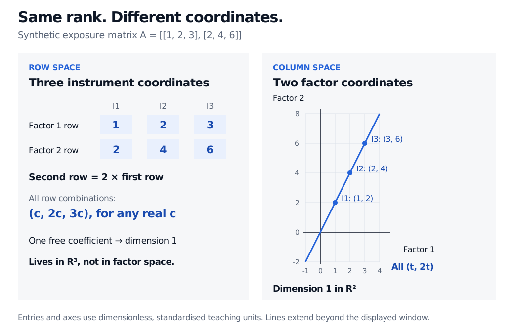
This is the line of achievable factor-exposure pairs in R2. The row space lives in R3, with instrument coordinates. Both spaces have dimension one, but they contain different kinds of vectors and belong to different ambient spaces.
The row space of A with rows 1, 2, 3 and 2, 4, 6 consists of all triples c, 2c, 3c in three instrument coordinates. Its dimension is one. The column space consists of pairs t, 2t in two factor coordinates, also dimension one; plotted columns are 1, 2; 2, 4; and 3, 6.
Original synthetic exposure example in dimensionless, standardised units. The left panel lists three coordinates; the right plots the two-dimensional factor space. Equal rank does not identify the two spaces.
What the exposure report cannot see
The null space, or kernel, contains holding changes z satisfying Az=0. Here
z1+2z2+3z3=0⟺z=s−210+t−301,s,t∈R.
Both basis vectors have zero dot product with (1,2,3): −2+2=0 and −3+3=0. Thus every null-space vector is perpendicular to every row-space vector. For any real matrix, using the ordinary Euclidean inner product,
Row(A)=ker(A)⊥,dimRow(A)+dimker(A)=n.
In this example the dimensions are 1+2=3. The general reason is visible in matrix multiplication: Az=0 says that every row has zero dot product with z. It is then perpendicular to every combination of those rows. Matching dimensions gives the full orthogonal-complement equality. MIT's orthogonality notes develop this relationship.
For example, holdings (1,1,0) produce exposures (3,6). Adding the null-space vector (−2,1,0) gives holdings (−1,2,0) and the same exposures (3,6).
These are zero-exposure changes under the stated matrix. They need not have zero purchase cost, zero realised profit and loss, or zero exposure to omitted factors. A local sensitivity model can also cease to match after a large market move. The algebra provides no standalone arbitrage conclusion. And orthogonality here concerns fixed coordinate vectors; it does not assert statistical independence of random returns or factors.
Why a minimum-norm solution sits in the row space
Every holding vector can be split uniquely into a row-space component and a null-space component. The exposure map sees only the first. For the target b=(3,6), the row-space solution must have the form wrow=c(1,2,3)⊤. Its first exposure is 14c, so
wrow=143123=3/143/79/14.
Every solution is wrow+z with z∈ker(A). Since the components are perpendicular,
∥wrow+z∥22=∥wrow∥22+∥z∥22.
The unique smallest Euclidean norm occurs at z=0. Its squared norm is 9/14, compared with 2 for (1,1,0).
That conclusion depends on the chosen standardised position coordinates. Rescaling instruments changes the meaning of this norm. Minimum Euclidean size does not automatically mean minimum cash cost, margin, turnover or portfolio variance; those need their own objectives and constraints.
Finding a row-space basis
Transpose the matrix and its rows become columns, giving Row(A)=Col(A⊤). For hand calculation, row reduction is usually more convenient: elementary row operations preserve the row space because they are reversible linear combinations of rows. The nonzero rows of an echelon form give a basis. Here subtracting twice row one from row two leaves (1,2,3) and a zero row. The zero row belongs to the space but contributes no basis vector.
Row reduction generally changes the column space. To find a column-space basis, take the pivot columns of the original matrix, rather than its row-reduced version. With rounded empirical loadings, distinguish exact row dependence from numerical rank under a declared tolerance and scaling.
For a worked route from free variables to kernel basis vectors, see Methods 1–2 of The Nullspace: Solving Ax = 0. The public page previews the lesson; the full lesson requires membership.
Sources
Gilbert Strang, Introduction to Linear Algebra, 5th edition, §§3.4–3.5 and §4.1 — row-space bases, dimensions of the four subspaces and orthogonal complements.